Different Types of Non-Preemptive CPU Scheduling Algorithms

CPU scheduling refers to the switching between processes that are being executed. It forms the basis of multiprogrammed systems. This switching ensures that CPU utilization is maximized so that the computer is more productive.

There are two main types of CPU scheduling, preemptive and non-preemptive. Preemptive scheduling is when a process transitions from a running state to a ready state or from a waiting state to a ready state. Non-preemptive scheduling is employed when a process terminates or transitions from running to waiting state.

This article will focus on two different types of non-preemptive CPU scheduling algorithms:
First Come First Serve (FCFS) and Shortest Job First (SJF).

First Come First Serve (FCFS)

As the name suggests, the First Come First Serve (FCFS) algorithm assigns the CPU to the process that arrives first in the ready queue. This means that the process that requests the CPU for its execution first will get the CPU allocated first. This is managed through the FIFO queue. The lesser the arrival time of processes in the ready queue, the sooner the process gets the CPU.

Advantages of FCFS algorithm

• It is the simplest form of a scheduling algorithm.
• Its implementation is easy and it is first-come, first-served.

Disadvantages of FCFS algorithm

• Due to the non-preemptive nature of the algorithm, short processes at the end of the queue have to wait for long processes that are present at the front of the queue to finish.
• There is a high average waiting time that causes a starvation problem.

A ready queue and Gantt chart should be used to perform this algorithm. But, before we dive into the details, let’s look at what a Gannt chart is.

Gantt chart

A Gantt chart is a bar chart that shows processes formed against time.
Here’s a numerical example for better understanding.

Solved numerical problem
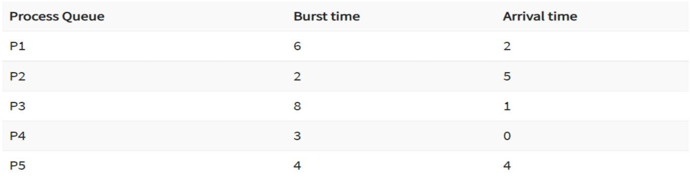
Consider the table with 5 processes and their burst and arrival times.

Burst and arrival time for different processes
Image source: Author

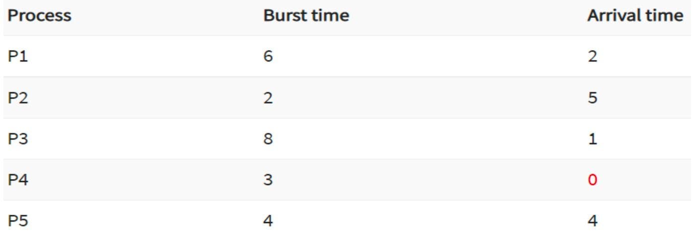
Burst and arrival time for different processes
Image source: Author

Before applying the FCFS algorithm, here’s a glimpse of the algorithm snippet for calculating average waiting time and average turnaround time.

C++ code snippet for FCFS algorithm
Image source: Author

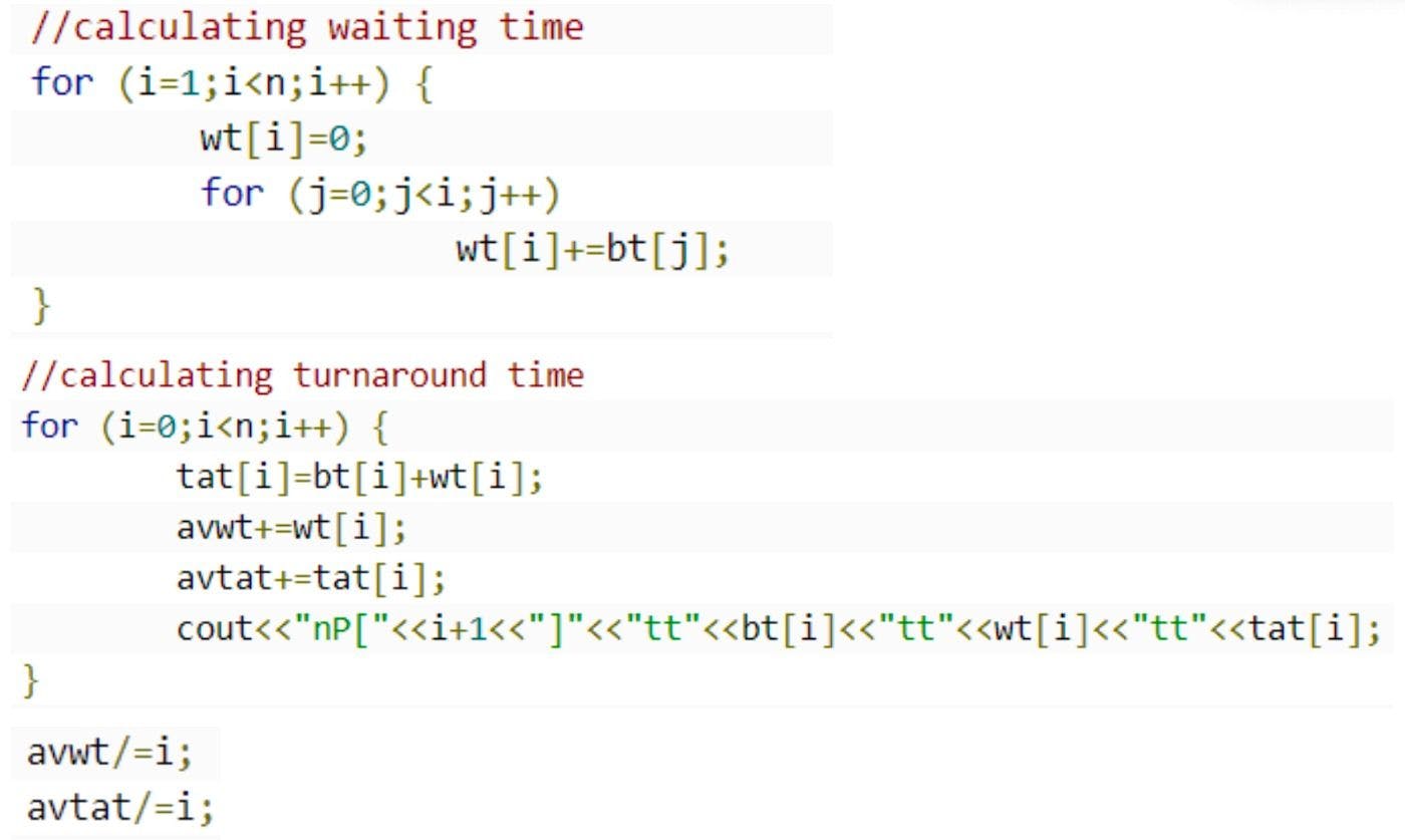
C++ code snippet for FCFS algorithm
Image source: Author

where, wt denotes waiting time, bt denotes burst time, tat denotes turnaround time, avwt denotes average waiting time, and avtat denotes average turnaround time.

Here’s another example.

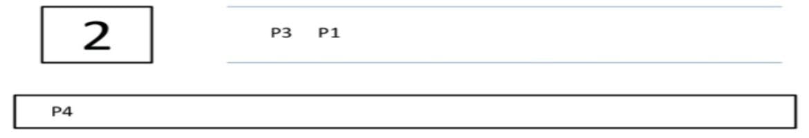
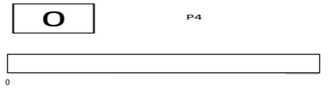
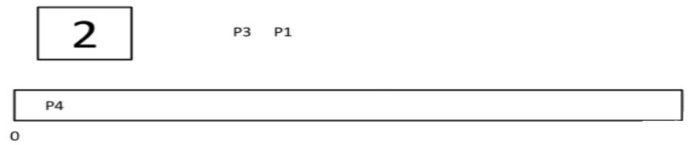
Step A: Process P4 has the least arrival time so it will enter the ready queue first. Until now, the Gantt chart is empty and initial time is 0.

Image source: Author

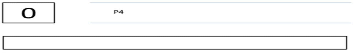
Image source: Author

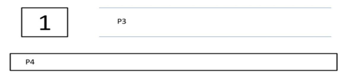
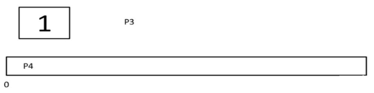
Step B: At time =1, P4 is still executing while P3 arrives so P3 will be kept in queue.

Image source: Author

Image source: Author

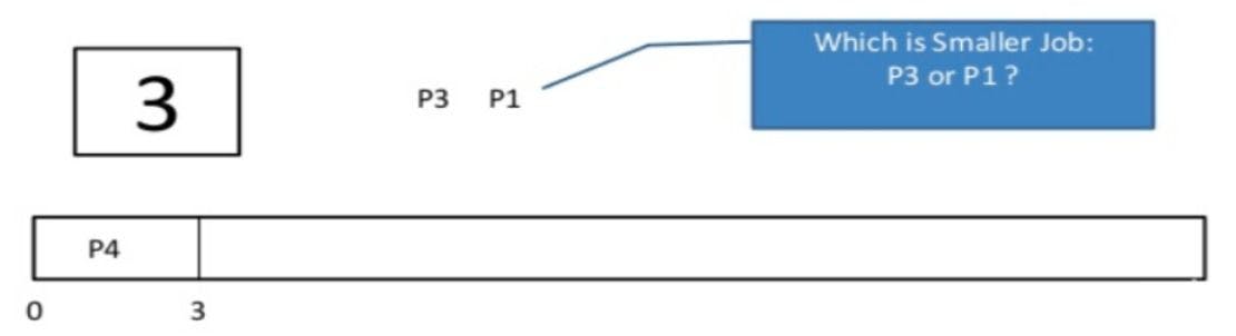
Step C: At time=2, P1 arrives but P4 is still executing so P1 is kept waiting in the ready queue.

Image source: Author

Image source: Author

Step D: At time=3, the burst time of P4 has been completed so the CPU is in IDLE state.

Image source: Author

Image source: Author

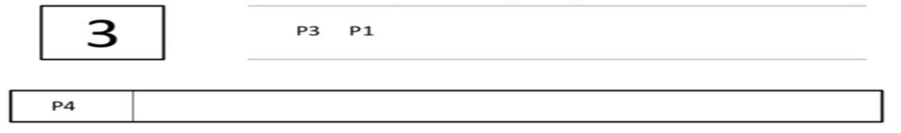
Step E: At time=4, the scheduler will pick up the process present in the front of the queue (P3) and pass it to the CPU for execution.

Image source: Author

Image source: Author

Step F: At time=5, P2 will arrive but as P3 is being executed, it’s kept waiting in the ready queue.

Image source: Author

Image source: Author

Step G: At time=11, the burst time of P3 is completed. It is fully executed by the CPU and will be terminated. The scheduler will then pick up P1 present in the front of the queue for execution.

Image source: Author

Image source: Author

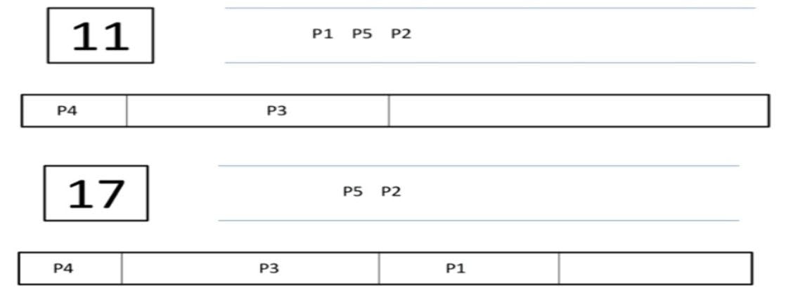
Step H: At time=17, the burst time of P1 is completed and is terminated. The scheduler will pick up P5 present in the front of the queue.

Image source: Author

Image source: Author

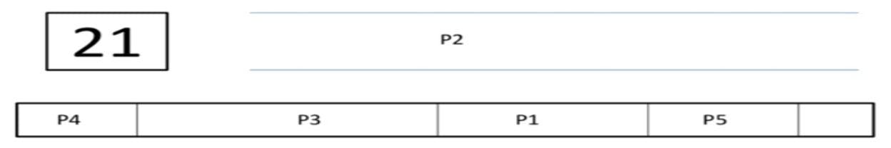
Step I: At time=21, the burst time of P5 is completed and terminated. The scheduler picks up P2 present in the front of the queue for execution.

Image source: Author

Image source: Author

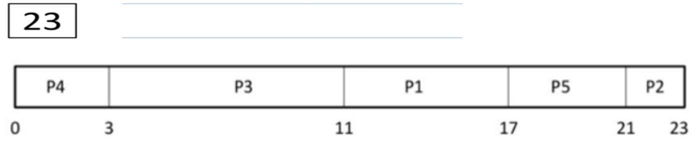
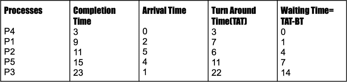
Here’s the completion time of all processes using the Gantt chart.

Image source: Author

Image source: Author

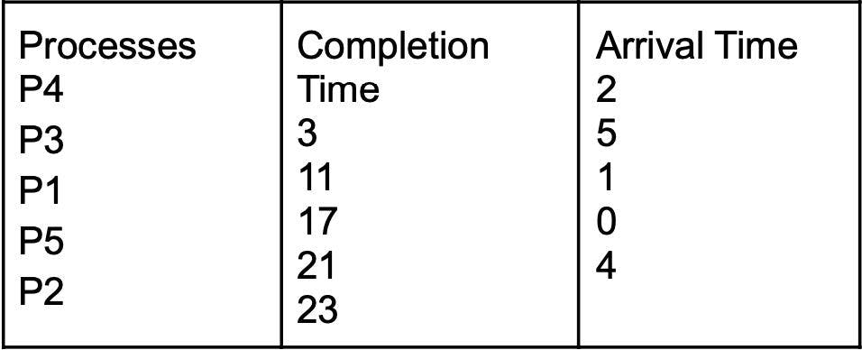
The final calculation for finding the average waiting time and turnaround time is as follows:

Image source: Author

Image source: Author

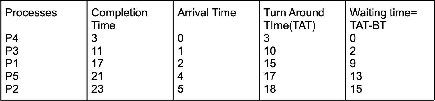
Average waiting time = (0+2+9+13+15)/5=7.8 ms.

Shortest Job First (SJF)

In the Shortest Job First (SJF) algorithm, the scheduler selects the process with the minimum burst time for its execution. This algorithm has two versions: preemptive and non-preemptive.

Advantages of SJF algorithm

• The algorithm helps reduce the average waiting time of processes that are in line for execution.
• Process throughput is improved as processes with the minimum burst time are executed first.
• The turnaround time is significantly less.

Disadvantages of SJF algorithm

• The SJF algorithm can’t be implemented for short-term scheduling as the length of the upcoming CPU burst can’t be predicted.

Solved numerical problem
Here’s a numerical example for better understanding.

Burst and arrival times for different processes
Image source: Author

Burst and arrival times for different processes
Image source: Author

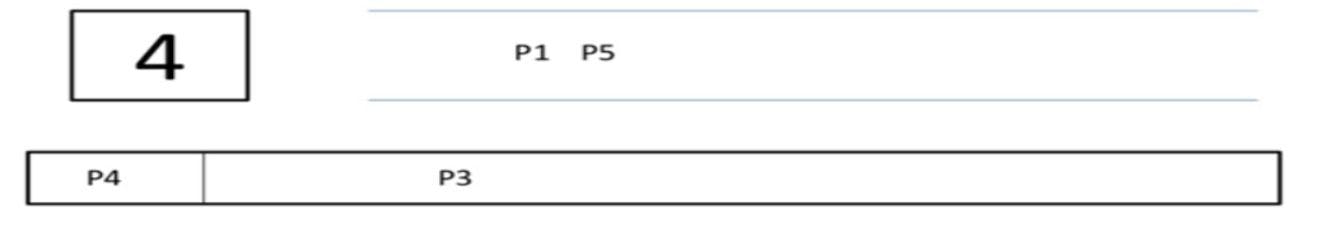
Step A: As process P4 has the least arrival time, it will enter the ready queue first. The initial time is 0 and the Gantt chart is empty until now.

Image source: Author

Image source: Author

Step B: At time =1, P4 is still executing while P3 arrives. Hence, P3 will be kept in the queue.

Image source: Author

Image source: Author

Step C: At time=2, P1 arrives but P4 is still executing so P1 is kept waiting in the ready queue.

Image source: Author

Image source: Author

Step D: At time=3, the burst time of P4 has been completed so the CPU is in IDLE state.

Image source: Author

Image source: Author

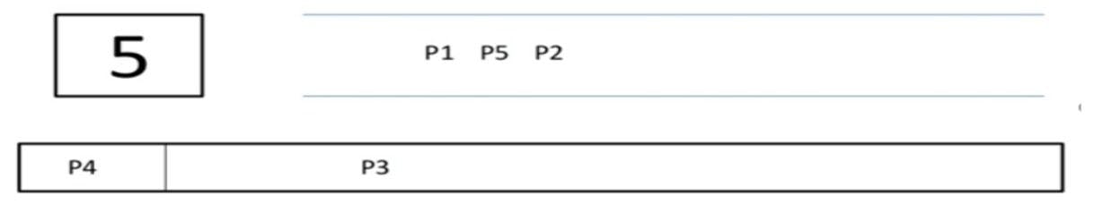
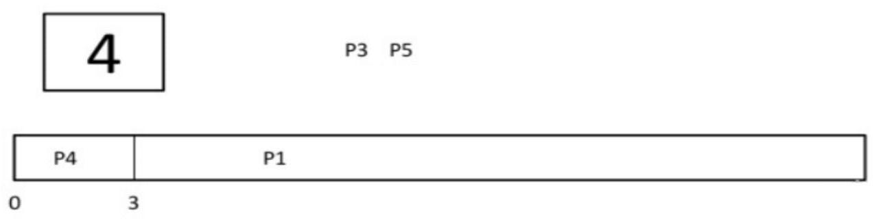
Step E: At time=4, the scheduler will pick up the process with the shorter burst time (P1) and pass it to the CPU for execution. P5 arrives in the ready queue.

Image source: Author

Image source: Author

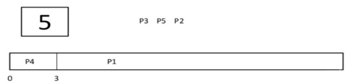
Step F: At time=5, P2 arrives but since P1 is already being executed, it’s kept waiting in the ready queue.

Image source: Author

Image source: Author

Step G: At time=9, the burst time of P1 is completed. It’s now fully executed by the CPU and will be terminated. The scheduler will then pick up the process with the minimum burst time. Since P2 has the lowest, it is the preferred choice.

Image source: Author

Image source: Author

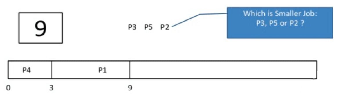
Step H: At time=10, P2 is still being executed.

Image source: Author

Image source: Author

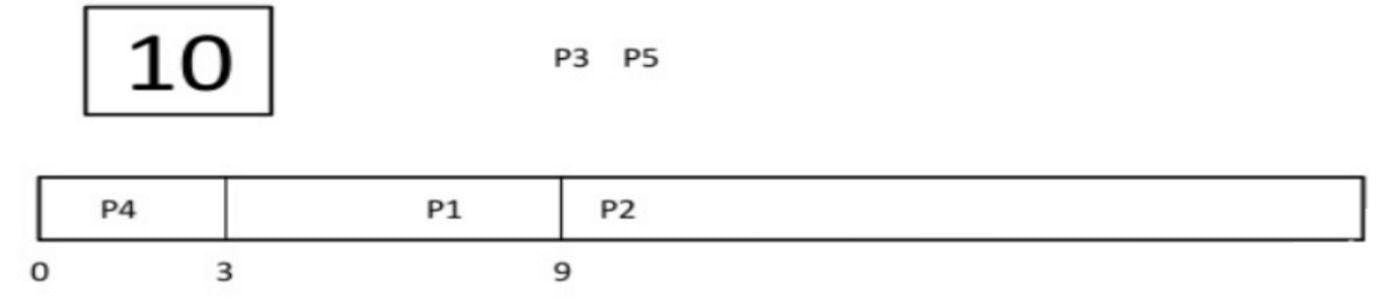
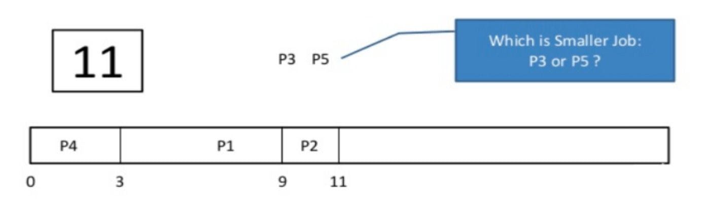
Step I: At time=11, the burst time of P2 is completed and it’s terminated. Again, the scheduler picks the process with the minimum burst time. In this case, it’s P5.

Image source: Author

Image source: Author

Step J: Finally, all the processes have arrived. At time=15, P5 will complete its execution and P3 will complete at time=23.

Image source: Author

Image source: Author

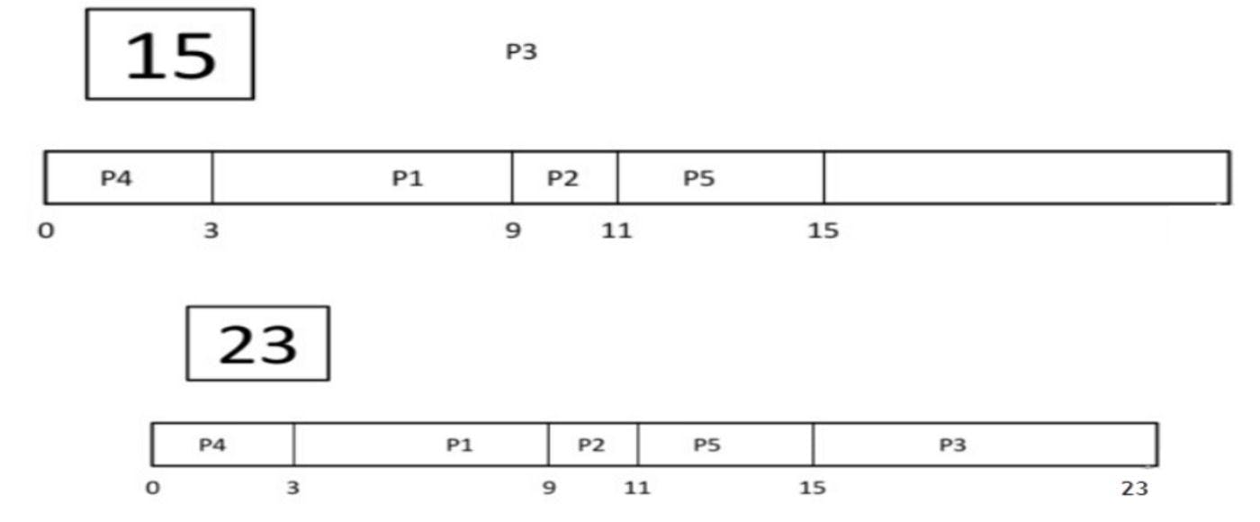
Here’s the completion time of the processes using the Gantt chart:

Image source: Author

Image source: Author

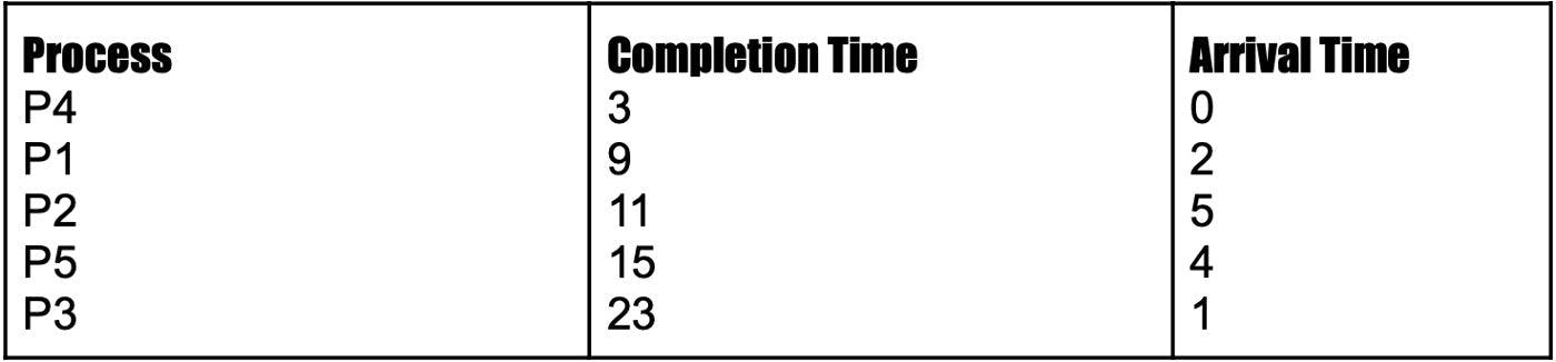
The final calculation for finding the average waiting and turnaround time is as follows:

Image source: Author

Image source: Author

The average waiting time=(0+1+4+7+14)/5=5.2ms.

You’ve now learned what you need to know about non-preemptive scheduling algorithms. Here’s a quick recap of a couple of key points:

i) The FIFO algorithm first executes the job that came in first in the queue.
ii) The Shortest Job First (SJF) algorithm minimizes the process flow time.