What is machine learning?

Machine learning is one of the areas of artificial intelligence (AI). It is defined as the study of programs that are not explicitly programmed, but instead, the algorithms learn patterns from data. It is where a computer program is said to learn from experience E with respect to some task T and some performance P if its performance on T, as measured by P, improves with experience E.

Over the last decade, ML has been adopted in different industries for various tasks, including breast cancer detection, building recommendation systems, and chatbots. The availability of large datasets and cheaper computing power has helped progress the growth of ML.

Types of machine learning systems

There are different types of machine learning systems, including:

Supervised learning

In supervised learning, the model is trained on labeled data. The most common supervised learning tasks are:

• Regression (predicting values)
• Classification (predicting classes).

Unsupervised learning

In unsupervised learning, the model is trained on unlabeled data and the algorithm learns to identify patterns.

Semi-supervised learning

In semi-supervised learning, the model is trained on labeled and unlabeled data, with most of the samples being unlabeled.

Reinforcement learning

In reinforcement learning, the model learns a policy by observing its environment where its actions are either rewarded or penalized.

Building a machine learning model step-by-step

In this section, we will understand how to build a machine learning model by following the workflow step-by-step.

Machine learning workflow

Problem statement and data collection

We will use the Bike sharing dataset which you can download here.
The data contains records of the number of bikes rented in a given hour and other features. We will use these features to build a model that can predict the number of bikes that will be rented.

The table below describes the features of the dataset.

Bike rental is affected by weather conditions and factors, such as whether it is a holiday.

Data exploration and preprocessing

Most machine learning practitioners agree that data exploration and preprocessing make up the majority of their work because available data may be incomplete or in a form that cannot be used directly.

Let us begin by loading the data into our notebook after importing some libraries that we will use.

import pandas as pd
import numpy as np
import matplotlib.pyplot as plt
import seaborn as sns

Load the data:

df = pd.read_csv("hour.csv")
df.head()

We can get a summary of the dataset using Panda's dataframe.info () method which shows the column names, the number of non-null rows, and their data types.

df.info()

Let us check if the dataset has any missing values to ensure they do not affect the model's overall performance.

df.isna().sum()

The data does not have missing values. However, the column names could be more informative. Let us rename them to more legible labels.

df.rename(columns={'instant':'record_id',
                        'dteday':'datetime',
                        'holiday':'is_holiday',
                        'workingday':'is_workingday',
                        'weathersit':'weather_condition',
                        'hum':'humidity',
                        'mnth':'month',
                        'cnt':'total_count',
                        'hr':'hour',
                        'yr':'year'},inplace=True)

Drop the ('record_id') because it does not contain any additional information about bike rentals. The 'casual' and 'registered' columns are combined to form the 'total_count' column; therefore, we can also drop these columns. This helps avoid data leakage, which happens when the training data contains information about the target variable that may not be available in the test set. In production, the model's performance will be affected.

 #the registered and casual columns are added to the total count
df. drop(['record_id','casual', 'registered'], axis=1, inplace=True)

The columns have different data types which we must convert to the most appropriate data type.

df['datetime'] = pd.to_datetime(df.datetime)
categorical variables
df['season'] = df.season.astype('category')
df['is_holiday'] = df.is_holiday.astype('category')
df['weekday'] = df.weekday.astype('category')
df['weather_condition'] = df.weather_condition.astype('category')
df['is_workingday'] = df.is_workingday.astype('category')
df['month'] = df.month.astype('category')
df['year'] = df.year.astype('category')
df['hour'] = df.hour.astype('category')

To understand the correlation between different features, create a correlation heat map. Such a map shows a correlation matrix between two dimensions. The Seaborn library is used to visualize the correlation map.

plt.figure(figsize=(12,8))
sns.heatmap(df.corr(), annot=True, cmap="Blues")

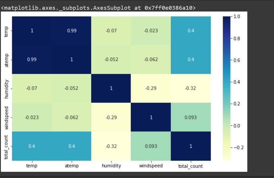
There is a high correlation between the temp and atemp features; therefore, we drop the 'atemp' column to avoid the effects of multicollinearity. Multicollinearity refers to where an independent variable can be predicted from another, making it difficult to determine the effects of each variable on the model. A deeper dive into multicollinearity is provided here.

df.drop('atemp', axis=1, inplace=True)

We will also drop the ‘datetime’ column
We have completed the data cleaning process and are ready to train our model.
First, we specify our features X and target variable Y and split the dataset into training and test sets. We use scikit-learn's train_test_split() method to split the dataset into 70% training and 30% test data.

from sklearn.model_selection import train_test_split

X = df.drop(['total_count'],axis=1)
y = df['total_count']
X_train, X_test, y_train, y_test = train_test_split(X,y, test_size=0.3, random_state=42)
X_train.shape, X_test.shape, y_train.shape, y_test.shape

Now, we can train our model.

Modeling: Training and testing

After preprocessing the data, we choose a machine learning algorithm to train and test the data on and make predictions. We use two algorithms employed in regression tasks: linear regression and random forest regression.

Linear regression is a parametric algorithm that finds the linear relationship between the features X and the target Y. It uses this relationship to predict the target variable given the dependent variables (features) during testing and production.

Learn more about the inner workings of linear regression here.

The scikit-learn library has several machine learning algorithms, including linear regression and random forest regression. We do not have to write them from scratch. We can import the algorithm and use the fit() and predict() methods to train the model and test, respectively.

import math  
import sklearn.metrics  
from sklearn.linear_model import LinearRegression
regressor = LinearRegression()
regressor.fit(X_train,y_train)
predictions = regressor.predict(X_test)
mse = sklearn.metrics.mean_squared_error(y_test, predictions)

rmse = math.sqrt(mse)
rmse

144.48157240539553

We test the performance of the model on the test dataset using the root mean square error (RMSE) which determines the accuracy of the model. A lower RMSE value indicates that the model makes fewer mistakes in its predictions.

Let us train the model with the same data using the random forest regression algorithm and compare the RMSE values.

from sklearn.ensemble import RandomForestRegressor

random_regressor = RandomForestRegressor()
random_regressor.fit(X_train, y_train)
preds = random_regressor.predict(X_test)
mean_error = sklearn.metrics.mean_squared_error(y_test, preds)

root_mean = math.sqrt(mean_error)
root_mean

42.5293221034906

The random forest regression model has a lower RMSE value; therefore, it is a better model compared to linear regression.

We will use the random forest regression model to build the ML pipeline. Note that you can experiment with other models to see how they perform and select the best.

The necessity of a machine learning pipeline

As observed from the steps above, the machine learning workflow involves several stages. They can be time-consuming, especially data cleaning and data processing. Every time we need to train the model with additional data, we have to repeat these steps. Hence, it is useful to automate the process.

A machine learning pipeline is a means of automating the end-to-end machine learning workflow. The ML pipeline uses the defined preprocessing steps on the supplied input to produce the expected output in each stage. ML pipelines can be implemented as a sequence of components where the ML workflow is split up into independent, reusable, modular parts that can then be combined to build models. This creates a more robust architecture for machine learning projects similar to the microservices architecture.

An ML pipeline can also be used as a single component for data preprocessing, taking data as input and predictions as output. Using a pipeline allows for effective data collection, data cleaning, and continuous training.

Machine learning pipeline example

Scikit-learn provides a built-in function for creating pipelines. The library offers two functions, sklearn pipeline and sklearn make_pipeline, which simplifies pipeline construction further. You can learn more about make_pipeline here and explore all the parameters of the sklearn pipeline in the documentation.

Below, we build a pipeline based on the data and steps we worked with previously.

1. Load the data
2. Perform data preprocessing
3. Split the data
4. Apply transformations to the data using the 'fit()' method
5. Make predictions and evaluate model performance.

The figure below shows the process in our pipeline:

Let us begin by importing the necessary packages and loading the dataset.

import pandas as pd
import numpy as np
df = pd.read_csv("hour.csv")

From the data exploration and data visualization we did previously, we know that some column names in our dataset need to be more descriptive and we need to rename them.

df.rename(columns={'instant':'record_id',
                        'dteday':'datetime',
                        'holiday':'is_holiday',
                        'workingday':'is_workingday',
                        'weathersit':'weather_condition',
                        'hum':'humidity',
                        'mnth':'month',
                        'cnt':'total_count',
                        'hr':'hour',
                        'yr':'year'},inplace=True)

Let us drop columns that we will not use in training the model.

df. drop(['record_id','casual', 'registered', 'datetime', 'temp'], axis=1, inplace=True)

The data is ready for model training. We will be using the random forest regression algorithm.

To create a pipeline, we import Pipeline from the scikit-learn package.

from sklearn.ensemble import RandomForestRegressor
from sklearn.model_selection import train_test_split
from sklearn.metrics import mean_squared_error
from sklearn.pipeline import Pipeline

We need to split the data into a training and test set.

X = df.drop(['total_count'],axis=1)
y = df['total_count']
X_train, X_test, y_train, y_test = train_test_split(X,y, test_size=0.3, random_state=42)

The Pipeline class takes several parameters:

class sklearn.pipeline.Pipeline(steps, *, memory=None, verbose=False)

Steps is a list of tuples of the transforms to be performed on the data. Each tuple consists of a name and a transform. The last transform must be an estimator - the machine learning algorithm which will be used for training and making predictions. The other parameters are optional depending on your specific implementation of scikit-learn pipelines.

In this example, the Pipeline class only has one tuple because the data preprocessing steps have already been implemented. This tuple will be used as the estimator.

pipeline = Pipeline(steps = [
            ('regressor',RandomForestRegressor())
           ])

Train the model using the fit() method, which uses the training dataset.

model = pipeline.fit(X_train, y_train)
print (model)

Make predictions using the predict() method and determine the model’s performance with the root mean square error metric.

predictions = model.predict(X_test)
print(math.sqrt(mean_squared_error(y_test,predictions)))

42.64736859923981

Here is the entire code used in this tutorial.

In this article, we learned to build a simple machine learning pipeline in Python with scikit-learn since our dataset did not need a lot of transformation to be used in training. We can build more complex pipelines depending on the transformations performed on the dataset, such as encoding categorical variables and replacing missing values.