What is a window function?

Before we proceed with this tutorial, let’s define a window function. A window function executes a calculation across a related set of table rows to the current row. It is also called SQL analytic function. It uses values from one or different rows to return a value for each row.

A distinct feature of a window function is the OVER clause. Any function without this clause is not a window function. Rather, it can be termed as a single-row function or an aggregate function.

Window functions make it easier to perform calculations and aggregations against multiple partitions of specific data. Unlike the single-row function that only returns a single value for each row defined in the query, window functions return a value for every single partition.

Why use window functions?

Window functions reduce complexity and increase the efficiency of queries that analyze cross-sections of data by providing a substitute to the usually complex SQL queries.

Here are some of the most common use cases of window functions:

• Accessing data from a different partition; for example, period-over-period inventory reporting.
• Ranking results within a window.
• Creating new features for machine learning models.
• Aggregation within a particular window; for instance, running totals.
• Imputing or interpolating missing values depending on the statistical characteristics of other values in the group.

If you have panel data, you will find that window functions are very useful when it comes to augmenting data with new features that characterize the aggregate properties of a particular data window.

Requirements to create a window function in SQL

In order to create a window function in SQL, the three parts below are required:

1. An aggregation calculation or function to apply to the particular column. For example, RANK(), SUM().
2. The PARTITION BY clause which defines the kind of data partition(s) to use in the aggregate function/calculation.
3. The OVER() clause to commence the window function.

In addition to the above three, you may also want to use the ORDER BY function to define the sorting required for each data window.

Pandas window function

When converting SQL window functions to Pandas, you should use the .groupby keyword instead of GROUP BY. .groupby is the cornerstone of Pandas window functions and is analogous to the SQL PARTITION BY command. The keyword specifies which parts or groups of the dataset should be used for the aggregation calculation/function.

The .transform clause will assist you in doing complex transformations. It allows you to provide the computation or aggregation that will be used to apply the dataset partitions. It accepts a function as an argument and returns a data frame of the same length as self. It is used to invoke a function on self that generates a series with transformed values that match the original's axis length.

The function used in transform() can be of the 'string' type; for example, for aggregation functions like ‘mean, 'count', 'sum', or a callable function for more complex operations like lambda function.

It's worth noting that you can only use transform() on aggregate functions that return a single row. This means that when dealing with a dataset that is not an aggregation function, you do not need to call transform().

Performing SQL-like window functions in Pandas Python

For this tutorial, we will utilize open-source time series data of stock prices of a group of companies.

Libraries and modules used

ffn (Financial functions for Python)

The library ffn has a lot of functions that are helpful for people who work in quantitative finance. It offers a wide range of utilities, from performance assessment and evaluation to graphing and common data transformations. It is built on top of popular Python packages like Pandas, NumPy, SciPy, etc.

Datetime

Classes for manipulating dates and times are available in the datetime module. Many different applications like time series analysis, stock analysis, banking systems, etc., require processing dates and times.

Depending on whether they contain timezone information, the date and time objects can either be categorized as aware or naive. We can use the date class of the datetime module after importing it. This class aids in the conversion of date attributes that are numerical to date format in the form of YYYY-MM-DD. Year, Month, and Day are the three properties that the class accepts in the following order (Year, Month, Day).

SQLite3

SQLite is an independent, file-based SQL database. Python already includes SQLite, so you can use it in all of your Python projects without installing any other programs. A standardized Python DBI API 2.0, conforming interface to the SQLite database, is provided by PySQLite. PySQLite is a suitable option if your application needs to handle MySQL, PostgreSQL, and Oracle in addition to the SQLite database.

random

random is a built-in Python module used to generate a series of random integers. These are unreal random numbers that lack actual randomness. We can create random integers using this module, show a random item from a list or string, and more.

Additionally, the random module offers the SystemRandom class, which creates random numbers from operating system-provided sources by calling the system method os.urandom().

Pandas

Pandas is arguably the most widely used library for working with data. Built on top of NumPy, it is an open-source Python library largely used for data analysis. It is an indispensable toolkit for Python data preparation, transformation, and aggregation. Users can take advantage of capabilities comparable to those in relational databases or spreadsheets by using tabular data structures that are exclusive to Pandas, Series and DataFrame.

Setup

The code below shows some simple configurations for gathering this dataset.

Step 1: Installing the necessary libraries

# install required libraries if necessary
!pip install datetime
!pip install random
!pip install ffn
!pip install sqlite3
!pip install pandas

Step 2: Importing libraries

Now, we import the required libraries for this demonstration.

import datetime
import random
import ffn
import sqlite3
import pandas as pd

Step 3: Collecting data

For this step, we will use the ffn library to collect our data. This popular Python library lets us collect data with just a single line of code.

stocks = [
    "AAPL",  
    "DIS",  
    "NKE",  
    "TSLA",  
]
getting the stock price dataset
P = ffn.get(stocks, start="2018-01-01")
using df.melt() to unpivot our data
P = P.melt(ignore_index=False, var_name="stocks", value_name="closing_price")
P = P.reset_index()
P.head()

Step 4: Saving the data to the SQLite database

The reason we are using the SQLite database is so that we can compare Pandas to SQL to gain more insight on how to use SQL in Python.

# connecting to an in-memory sqlite database
with sqlite3.connect(":memory:") as conn:
# saving our dataframe to sqlite database
    P.to_sql(name="P", con=conn, index=False)

From here, we have SQL in Python. We can now perform SQL-like window functions, but in Python.

Calculating stock prices in Pandas

In the next step of this tutorial, we will calculate the following in Pandas:

• The max stock price for individual companies over the same period.
• Moving average of the 28-day closing price for individual companies.
• Previous day’s closing price share for individual tickers.
• Daily percentage return.
• Missing data interpolation.

Max stock price for individual companies

To perform this function, we will utilize groupby to partition the dataset by ticker and introduce max to the transform() to create a new column for displaying the maximum share price for the ticker.

A very important point to note: since max is a simple calculation/aggregation function, you can simply pass it as a string to transform (), rather than calling a new function. This is the beauty of SQL in Python!

df1 = P.copy()
adding a new column
df1["max_price"] = df1.groupby("stocks")["closing_price"].transform("max")
df1

Moving average of the 28-day closing price

In this section, we will create a new partition in the dataframe and call it ‘ma_28-day’ using both groupby () and transform (). To apply Pandas SQL query on DataFrame, we will use lambda syntax to define the type of function to be applied to the individual groups.

# copy original dataframe (optional)
df2 = P.copy()
adding a new column
df2["ma_28_day"] = (
df2.sort_values("Date")
.groupby("stocks")["closing_price"]
.transform(lambda x: x.rolling(28, min_periods=1).mean())
)
df2

Previous day’s closing price share for individual ticker

Since the shift clause automatically returns a value for each partition in the data, we don't have to use transform ().

df3 = P.copy()
df3["previous_close"] = (
df3.sort_values("Date").groupby("stocks")["closing_price"].shift(1)
)
df3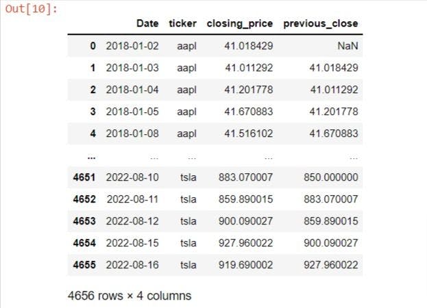

Daily percentage return

For this operation, we will call the lambda function syntax due to the complexity of the calculation required in each partition.

df4 = P.copy()
df4["daily_return"] = (
df4.sort_values("Date")
.groupby("stocks")["closing_price"]
.transform(lambda z: z / z.shift(1) - 1)
)
df4

Missing data interpolation

For this example, Pandas is probably more efficient than SQL in using window-type functions for missing data interpolation.

To begin, we will randomly slice out some data to simulate absent data in the actual dataset. From there, we will use imputation() or interpolation() to load the missing data within each group with numbers that resemble the rest of the dataset.

For this case, we will utilize the ‘forward fill’ technique to assign the data of the previous closing share price if the value is missing.

The Pandas SQL query example is as follows:

df5 = P.copy()
# removing 30% of the data
pct_removed = 0.3
num_removed = int(pct_removed * len(df5))
ind = random.sample(range(len(df5)), k=num_removed)
new_val = [k in ind for k in range(len(df5))]
inserting missing data
df5["closing_price_interpolated"] = (
df5.sort_values("Date")
.groupby("stocks")["closing_price"]
.transform(lambda x: x.interpolate(method="ffill"))
)
df5

# checking for missing data
df5.isnull().sum()

SQL in Python gives data scientists the flexibility of being able to perform data transformation in either Pandas or SQL. It allows analysts to quickly move between tools and datasets without having to relearn the syntax of each.

One of the challenges of implementing this module was creating a common framework for mapping SQL data types to Python data types. This framework simplifies the translation of an SQL query into a Pandas DataFrame. While each language will have a varying degree of complexity depending on the dataset, it is still important to acquire competence in both and learn how window functions can be performed in Pandas and SQL.

Once a query has been created using SQL, it can be translated into a Pandas DataFrame by either manually creating columns from the table, by using the Pandas built-in function sqlmap, or by using an external module like sqlite3. If a table is created in Pandas, a number of functions that can be used in SQL can also be used in Pandas, as we saw in this tutorial.