Understanding a Confusion Matrix and How to Plot It

Have you faced a situation where you expected a machine learning model to perform as anticipated but for some reason, it lagged? You did all the hard work and programming but the classification model just could not perform to par. How can you correct this?

There are several ways to gauge the performance of a classification model but none quite like the confusion matrix. This unique matrix evaluates how the model performs and where it faces issues in order to help developers streamline development.

In this article, we will look at confusion matrices and learn how to use them to determine the performance matrix in ML classification issues.

What is a confusion matrix?

A confusion matrix is an N X N matrix that is used to evaluate the performance of a classification model, where N is the number of target classes. It compares the actual target values against the ones predicted by the ML model. As a result, it provides a holistic view of how a classification model will work and the errors it will face.

Running a classification model produces two outcomes:

• Binary 0
• Binary 1

where 0 means False and 1 means True.

Based on these two outcomes, we can easily compare the resulting classification outcomes with the actual values of the observation. This helps in judging the performance of a classification model. The matrix used in these outcomes is known as the confusion matrix.

Here is how it works:

Image source

Image source

Let’s decipher the matrix and appreciate its parameters and outcomes.

Understanding TP, TN, FP, and FN outcomes in a confusion matrix

There are four potential outcomes:

1. True positive
2. True negative
3. False positive
4. False negative

True positive (TP) is the number of true results when the actual observation is positive.

False positive (FP) is the number of incorrect predictions when the actual observation is positive.

True negative (TN) is the number of true predictions when the observation is negative.

False negative (FN) is the number of incorrect predictions when the observation is negative.

We already know that a confusion matrix is used to measure the performance indicators for classification models. Let’s now understand the four main parameters that play a vital role in it.

Precision

Precision is the analysis of the true positives over the number of total positives that are predicted by the machine learning model. The formula for precision is written as TP/(TP+FP). This indicator allows you to calculate the rate at which your positive predictions are actually positive.

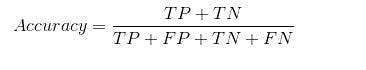
Accuracy

Accuracy is the most commonly used parameter that is employed to judge the machine learning model. For example, if 70% of cases are false and only 30% are true then there is a high possibility of the ML model having an accuracy score of 70%. The formula to calculate accuracy is (TP+TN)/(TP+FP+FN+TN).

Recall

Sensitivity or recall is the measure of the TP over the count of the actual positive outcomes. The formula to calculate Recall is TP/(TP+FN). This parameter assesses how well the ML model can analyze the input and identify the actual result.

F1 score

The harmonic mean of precision and recall is the F1 score. It is used as an overall indicator that incorporates both precision and recall. This harmonic mean analyzes both false positives and false negatives and performs well on an imbalanced dataset. The formula to calculate it is 2(p*r)/(p+r), where r is the recall and p is precision.

Which performance indicator should you use and when?

A simple question with a fairly simple answer: it depends. There is nothing like a one-size-fits-all solution as these parameters are important in their own ways. They provide different pieces of information about the performance of the classification model.

Let’s look at how these performance indicators play a crucial role in plotting a confusion matrix.

- Accuracy: Accuracy is usually not a great performance indicator for the overall ML model performance. It can be used to compare the model outcomes while converting training data and finding the optimal values for an actual result.

- Precision: Precision calculates the predicted positive rate. It is a good indicator to use when you want to focus on reducing false positives.

A prime example of precision can be seen in disaster relief, including efforts and rescues. In a situation of disaster relief and rescue, you could make 100 rescues though there could be 100+ rescues needed to save everyone. If you’re working as part of a relief effort and know this, you need to ensure that the rescues you make are true positives and that you are not wasting precious resources and time.

- Recall: The recall is a measure of a true positive rate. It is an appropriate metric to use when you focus on limiting false negatives. It is employed in medical diagnostics and other related tests, such as for COVID-19. The chances of risks are greater. You will see an increase in the number of infected and carriers spreading it to others. The infected will believe that they are negative due to false-negative tests.

- F1 score: The F1 score limits both the false positives and false negatives as much as possible. The parameter is used in different general performance operations unless the issue specifically demands using precision or recall.

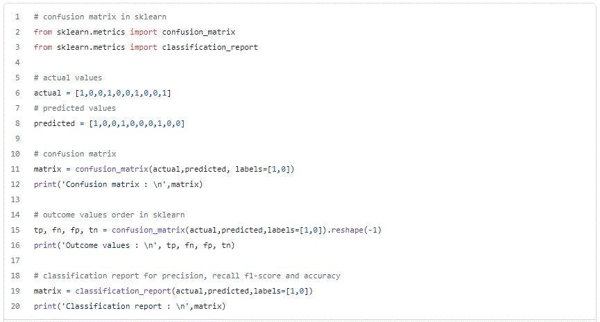
Here, we will learn how to plot a confusion matrix with an example using the sklearn library. We will also learn how to calculate the resulting confusion matrix.

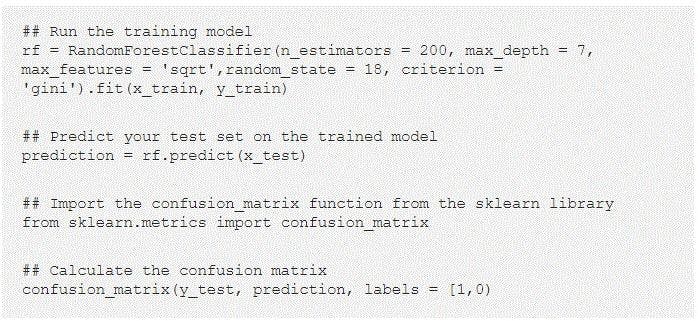
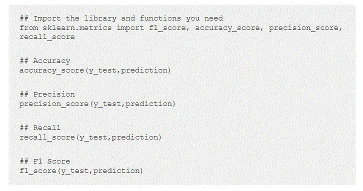
The model predicts the data once it is successfully trained. In the confusion matrix example, we can see that TP = 66, FP = 5, FN = 21, and TN = 131.

Calculating the different parameters:

Accuracy: (66+131)/(66+5+21+131) = 0.8834
Precision: 66/(66+5) = 0.9296
Recall: 66/(66+21) = 0.7586
F1 score: 2(0.9296*0.7586)/(0.9296+0.7586) = 0.8354

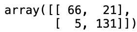
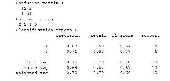
We have just seen a confusion matrix example using some values. Now, we will confirm the results and see how we can calculate the metrics with sklearn.

Code fragment:

Output:

Image source

Image source

Why do you need a confusion matrix?

Let’s take a hypothetical example of a classification issue before we answer this big question.

Let’s assume we want to predict the exact number of infected people and isolate them from the healthy population. According to the situation, the two values for our target variables would be Not Sick and Sick.

To better understand the reason behind having a confusion matrix, we take an example of an imbalance datasheet, with exactly 947 data points for the negative class and 3 data points for the positive class.

Calculating the accuracy:

Image source

Image source

Using the above formula for accuracy, let’s check how our model performed.

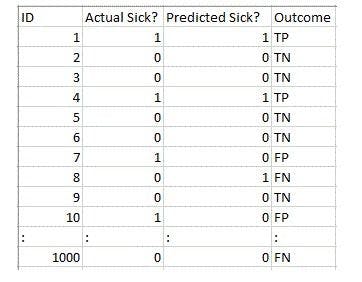
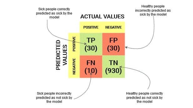
The total outcome values are:

True Positives = 30
True Negatives = 930
False Positives = 30
False Negatives = 10

So, our result comes out to be:

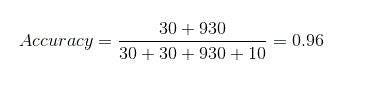
96% appears great but in reality, it is the opposite. Accuracy is actually showing the percentage of people who will not get sick with almost 96% accuracy, while the infected are spreading the virus.

This is where we incorporate the other performance metrics of a confusion matrix. We can understand the situation better with the help of a diagram.

Using recall and precision, we can see the actual results.

Image source

Image source

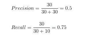
The correctly predicted cases are 50% of the total positive cases. On the other hand, our model predicted 75% of the positive cases.

Confusion matrix in Python

Now that we understand a confusion matrix, let’s learn how to plot it in Python using the Scikit-learn library.

Image source

Confusion matrix in Machine Learning

A confusion matrix in machine learning helps with several aspects and streamlines the model.
Here are a few reasons why we should plot it:

• When a classification model predicts the test data, a confusion matrix evaluates the performance and analyzes the efficiency of the model.
• It predicts the errors and their exact types, such as Type-I or Type-II.
• It helps in calculating the different parameters (accuracy, precision, recall)) of the model.

Features of a confusion matrix

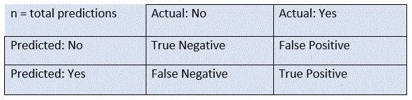
• For 2 classes, the matrix table is 2X2 and for 3 classes, it is 3X3, and so on.
• The entire matrix is bifurcated into two main dimensions, comprising the actual values along with the total number of predictions and the predicted values.
• The actual values are the true values for the considered observations and the predicted values are the values predicted by the model.

These features can be better understood with the image below.

Image source

Image source

Now that you’ve learned how to plot a confusion matrix, you can use it for data prediction in machine learning models.

Unlike its name suggests, the confusion matrix is far from confusing - once you know the basics. It is powerful and helps with predictive analysis, enabling you to analyze and compare predicted values against the actual values.