What Are the Regression Analysis Techniques in Data Science?

Why are regression analysis techniques needed?

Regression analysis helps organizations to understand what their data points mean and to use them carefully with business analysis techniques to arrive at better decisions. It showcases how dependent variables vary when one of the independent variables is varied and the other independent variables remain unchanged. It acts as a tool to help business analysts and data experts pick significant variables and delete unwanted ones.

Note: It’s very important to understand a variable before feeding it into a model. A good set of input variables can impact the success of a business.

Image source: Analytics Vidhya

Types of regression techniques

There are several types of regression analysis, each with their own strengths and weaknesses. Here are the most common.

Linear regression

The name says it all: linear regression can be used only when there is a linear relationship among the variables. It is a statistical model used to understand the association between independent variables (X) and dependent variables (Y).

The variables that are taken as input are called independent variables. In the example of the gym supplement above, the prices and advertisement effect are the independent variables, whereas the one that is being predicted is called the dependent variable (in this case, ‘sales’).

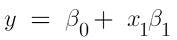
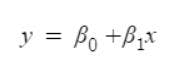
Simple regression is a relationship where there are only two variables. The equation for simple linear regression is as below when there is only one input variable:

If there is more than one independent variable, it is called multiple linear regression and is expressed as follows:

where x denotes the explanatory variable. β1 β2…. Βn are the slope of the particular regression line. β0 is the Y-intercept of the regression line.

If we take two variables, X and Y, there will be two regression lines:

• Regression line of Y on X: Gives the most probable Y values from the given values of X.
• Regression line of X on Y: Gives the most probable X values from the given values of Y.

Usually, regression lines are used in the financial sector and for business procedures. Financial analysts use regression techniques to predict stock prices, commodities, etc. whereas business analysts use them to forecast sales, inventories, and so on.

How is the best fit line achieved?

The best way to fit a line is by minimizing the sum of squared errors, i.e., the distance between the predicted value and the actual value. The least square method is the process of fitting the best curve for a set of data points. The formula to minimize the sum of squared errors is as below:

where yi is the actual value and yi_cap is the predicted value.

Assumptions of linear regression

• Independent and dependent variables should be linearly related.
• All the variables should be independent of each other, i.e., a change in one variable should not affect another variable.
• Outliers must be removed before fitting a regression line.
• There must be no multicollinearity.

Polynomial regression

You must have noticed in the above equations that the power of the independent variable was one (Y = m*x+c). When the power of the independent variable is more than one, it is referred to as polynomial regression (Y = m*x^2+c).

Since the degree is not 1, the best fit line won’t be a straight line anymore. Instead, it will be a curve that fits into the data points.

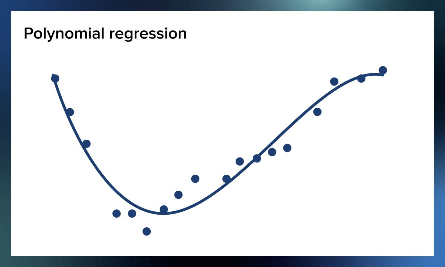
Image source: Serokell

Important points to note

• Sometimes, this can result in overfitting or underfitting due to a higher degree of the polynomial. Therefore, always plot the relationships to make sure the curve is just right and not overfitted or underfitted.

Image source: Analytics Vidhya

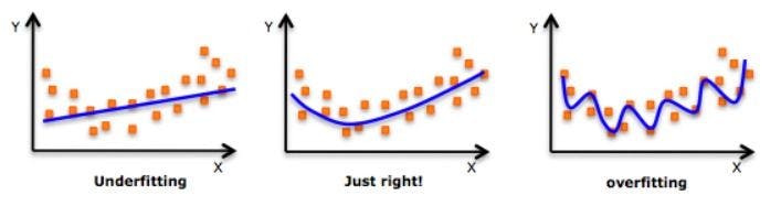
• Higher degree polynomials can end up producing bad results on extrapolation so look out for the curve towards the ends.

Logistic regression

Logistic regression analysis is generally used to find the probability of an event. It is used when the dependent variable is dichotomous or binary. For example, if the output is 0 or 1, True or False, Yes or No, Cat or Dog, etc., it is said to be a binary variable. Since it gives us the probability, the output will be in the range of 0-1.

Let’s see how logistic regression squeezes the output to 0-1. We already know that the equation of the best fit line is:

Since logistic regression analysis gives the probability, let’s take probability (P) instead of y. Here, the value of P will exceed the limits of 0-1. To keep the value inside this range, we take the odds of the above equation which will become:

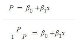
Another issue here is that the above equation will always give the output in the range of (0, +∞). We don’t want a restricted range because it may decrease the correlation. To solve this, we take log odds with a range of (-∞, +∞).

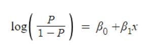
Since we want to predict the probability of P, we will simplify the above equation in terms of P and get:

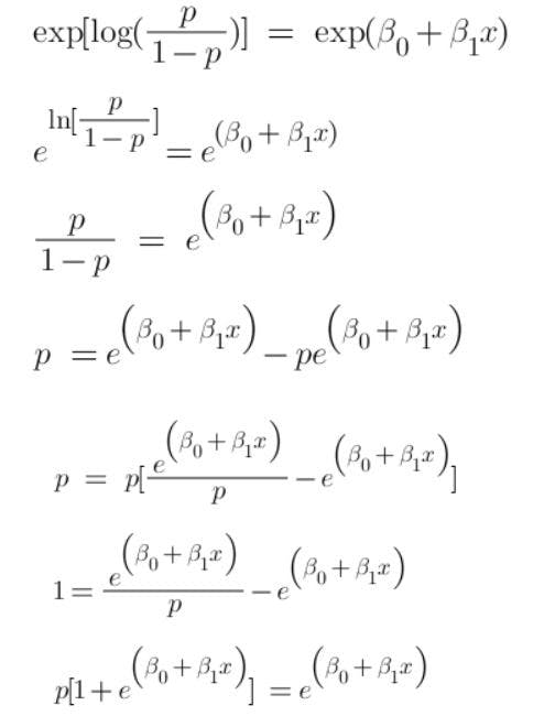
This is also called logistic function. The graph is shown below:

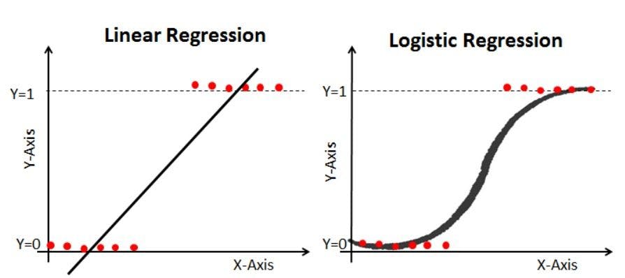
Image source: Datacamp

Important points to note

• Logistic regression is mostly used in classification problems.
• Unlike linear regression, it doesn’t require a linear relationship among dependent and independent variables because it applies non-linear log transformation to the predicted odds ratio.
• If there are various classes in the output, it is called multinomial logistic regression.
• Like linear regression, it doesn’t allow multicollinearity.

Ridge regression

Before we explore ridge regression, let’s examine regularization, a method to enable a model to work on unseen data by ignoring less important features.

There are two types of regularization techniques, ridge and lasso regression/regularization.

In real-world scenarios, we will never see a case where the variables are perfectly independent. Multicollinearity will always occur in real data. Here, the least square method fails to produce good results because it gives unbiased values. Their variances are large which deviates the observed value far from the true value. Ridge regression adds a penalty to the model with high variance, thereby shrinking the beta coefficients to zero which helps avoid overfitting.

In linear regression, we minimize the cost function. Remember that the goal of a model is to have low variance and low bias. To achieve this, we add another term in the cost function of linear regression: “lambda” and “slope”.

The equation of ridge regression is as follows:

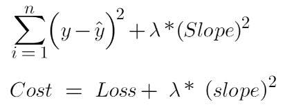
If there are multiple variables, we can take the summation of all the slopes and square it.

Lasso regression

Lasso or least absolute shrinkage and selection operator regression is very similar to ridge regression. It is capable of reducing the variability and improving the accuracy of linear regression models. In addition, it helps us perform feature selection. Instead of squares, it uses absolute values in the penalty function.

The equation of lasso regression is:

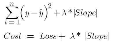
In the ridge regression explained above, the best fit line was finally getting somewhere near zero (0). The whole slope was not a straight line but was moving towards zero. However, in lasso regression, it will move towards zero. Wherever the slope value is less, those features will be removed. This means that the features are not important for predicting the best fit line. This, in turn, helps us perform feature selection.

How to select the right regression analysis model

The regression models discussed here are not exhaustive. There are many more, so which to choose can be confusing. To select the best, it’s important to focus on the dimensionality of the data and other essential characteristics.

Below are some factors to note when selecting the right regression model:

1. Exploratory data analysis is a crucial part of building a predictive model. It is and should be the first step before selecting the right model. It helps identify the relationship between the variables.
2. We can use different statistical parameters like R-square, adjusted square, area under the curve (AUC), and receiver operating characteristic (ROC) curve to compare the soundness of fit for different models.
3. Cross-validation is a good way to evaluate a model. Here, we divide the dataset into two groups of training and validation. This lets us know if our model is overfitting or underfitting.
4. If there are many features or there is multicollinearity among the variables, feature selection techniques like lasso regression and ridge regression can help.

Regression analysis provides two main advantages: i) it tells us the relationship between the input and output variable, ii) it shows the weight of an independent variable’s effect on a dependent variable.

The base of all the regression techniques discussed here is the same, though the number of variables and the power of the independent variable are increased. Before using any of these techniques, consider the conditions of the data. A trick to find the right technique is to check the family of variables, i.e., if the variables are continuous or discrete.