What is anomaly detection?

Anomaly detection involves the identification of infrequent occurrences that significantly differ from the majority of the data.

The application of anomaly detection in time series encompasses a wide range of practical uses such as manufacturing and healthcare. Anomalies indicate unexpected events that may arise from production errors or system malfunctions. For instance, if we monitor website visitors and observe a sudden drop to zero, it could indicate server failure.

Detecting anomalies in time series data is valuable when preparing for forecasting. Numerous forecasting models rely on autoregressive methods, wherein past values contribute to predictions. An outlier in the past will inevitably impact the model. Thus, removing such an outlier can enhance the accuracy of forecasts.

Anomaly detection algorithms

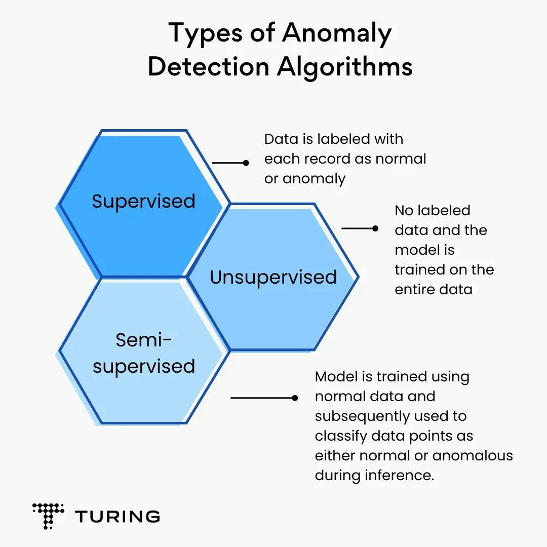
There are three broad categories of anomaly detection algorithms:

1. Supervised algorithm: This is a kind of algorithm in which data is labeled with each record as normal or anomaly.

2. Unsupervised algorithm: This type of data does not have labeled data and the model is trained on the entire data.

3. Semi-supervised algorithm: This algorithm follows a two-step process. The model is first trained using normal data. It is then applied to classify data points as either normal or anomalous during the inference phase.

Let’s take a look how we can achieve time series anomaly detection:

STL decomposition

STL, which stands for Seasonal and Trend decomposition using Loess, is a decomposition technique employed to analyze time series data. The technique breaks down the entire time series into three distinct components: trend, seasonality, and residual.

Each of these components is described as follows:

1. Trend: The trend component of a time series refers to the long-term increase or decrease in values over a specific period. It can manifest as either exponential or linear growth and has the potential to change direction over time.

2. Seasonality: Seasonality represents the repetitive pattern of values within a time series. These values exhibit a consistent trend that repeats after a regular interval such as hourly, weekly, monthly, or yearly.

3. Residual: Residual is defined as the noise present in the data. It signifies an unusual occurrence or an outlier that cannot be predicted or explained by the underlying trend or seasonal pattern.

The residual component captures the irregularities or unexpected variations in the data that are not accounted for by the trend or the seasonality. It represents the random and unpredictable elements of the time series.

For example, if there is an abrupt and uncharacteristic spike in sales during a particular month in a specific year, which is not observed consistently in other years, this anomalous behavior is considered as noise or a residual.

By decomposing a time series into these three components, STL facilitates a more comprehensive understanding of the underlying patterns and dynamics within the data. This decomposition can be utilized for various purposes including forecasting, anomaly detection, and data analysis.

STL decomposition using the statsmodel library:

Step 1. Install the statsmodel library

Install the statsmodels library using the following command:

pip install statsmodels

Step 2. Implement code

Implement the code to get the trend, seasonality, and residual graph of the data.

from stldecompose import decompose, forecast
import pandas as pd
data= pd.read_csv("timeseries.csv")
temp = data.reset_index()
df_month = temp[['index', 'timeseries']].set_index('index')
decomp = decompose(df_month.values, period=12)
trend = decomp.trend
seasonal = decomp.seasonal
residual = decomp.resid

Upon comparing the results obtained from both techniques, it is evident that there is a notable difference in the trend and residual components, while the seasonal component remains unchanged.

Clustering-based unsupervised approach

Unsupervised algorithms are useful when there is no labeled data. In such cases, clustering algorithms are very handy and are widely used in time series anomaly detection.

There are several popular clustering algorithms like KNN and K-Means, but they require the number of clusters to be defined beforehand. To overcome this challenge, there is a robust algorithm for time series anomaly detection that can be used: DBSCAN.

DBSCAN stands for Density-Based Spatial Clustering of Applications with Noise. The unsupervised algorithm accepts a multidimensional vector as input. It groups all the data points that are densely located in a region as one cluster.

Unlike KNN or K-means, it does not require the number of clusters as the input parameter; rather it needs two parameters, epsilon and MinPoint.

Epsilon is required to define the radius of the circle around each data point to check the density of data points within that circle. MinPoints defines the minimum data points that should be present within the circle to be considered a cluster.

Points that are not covered in the cluster are marked as outliers and can be defined as the anomaly.

DBSCAN algorithm using the Pandas library from scikit-learn:

from sklearn.cluster import DBSCAN
import pandas as pd
dbscan=DBSCAN()
df=pd.read_csv("data.csv")
dbscan.fit(df[["feature1", "feature2"]])

Autoregressive integrated moving average (ARIMA)

The ARIMA model can be used for real-time anomaly detection. It is widely used to forecast data points from the previous or historical data points.

It comprises three parts: autoregressive model (AR), integrated (I) and moving average (MA) which are explained below:

1. Autoregressive (AR) component: This component of the model determines the degree of relationship between the present value and the previous values. The AR component allows us to account for the autoregressive behavior or trend in the data.

2. Integrated (I) component: Most time series data is non-stationary and has seasonality present within the data. This seasonality trend has to be removed otherwise it will introduce bias in the model.

To overcome the challenge, the integrated component is introduced which involves taking the difference between consecutive observations to eliminate any underlying trend or seasonality.

3. Moving average (MA): This component determines the dependency between the current observation and the residual errors resulting from the previous observations. Residual errors are calculated by subtracting the predicted values from the actual values.

For each observation, we take a weighted average of the two most recent residual errors, giving more weight to the more recent one. The weights are determined by the coefficients associated with the MA component. Finally, we add the weighted average to the model's predictions to obtain the final forecast for the current observation.

Implementation of ARIMA model:

Step 1: Import all necessary libraries.

import pandas as pd
import numpy as np
import matplotlib.pyplot as plt
from statsmodels.tsa.arima.model import ARIMA

Step 2: Load ARIMA model.

data = pd.read_csv('your_data_file.csv')
train_size = int(len(data) * 0.8)  # 80% for training, 20% for testing
train_data = data[:train_size]
test_data = data[train_size:]
Create and fit the ARIMA model
model = ARIMA(train_data, order=(p, d, q))

model_fit = model.fit()
Perform predictions
predictions = model_fit.predict(start=len(train_data), end=len(train_data) + len(test_data) - 1)

Conclusion

In this article, we discussed the applications of detecting anomalies in data in healthcare and manufacturing. We also discussed algorithms like ARIMA, DBSCAN, and STL decomposition along with their implementation for anomaly detection.

Anomaly detection is important in time series data as it can be used to determine uncharacteristic trends in the data. In the case of machines, it is very important to detect failure of machine parts in advance. Anomaly detection can help identify such failures for predictive maintenance.