How to Develop Random Forest Ensemble in Python

Random forest. The name itself says it all. A forest with several trees.

Before we dive into a technical definition of a random forest algorithm, let’s understand it with a real-time example.

A real-time analogy of random forest algorithm

John wants to know all his professional career options after graduation. So, he asks for recommendations from a few of his seniors who studied in the same stream and are successfully working in the industry. Each one of them asks him questions about his interests and skills to know which career would suit him better.

Based on the answers given by John, each of them came up with an answer. He finally decides on a career that most of his seniors recommended.

Before we dig deep into the topic, let’s explore how to develop a random forest ensemble in Python. We will learn a random forest algorithm from scratch, its ensemble methods, and how it works. We will also provide code examples for practical understanding.

Random forest algorithm

To summarize it in technical terms, random forest is a supervised machine learning algorithm. It is used widely for classification and regression problems in machine learning. Based on the concept of ensemble learning, random forest combines various random forest classifiers and provides answers to complex problems.

The below given pictorial will further clarify the same.

Consider a dataset X. The algorithm, being a classifier, contains a number of decision trees on distinct subsets. It takes the prediction from each tree and offers the final output based on the majority votes of predictions. The more the number of trees, the more accurate the results are. It also avoids overfitting.

Image source

Image source

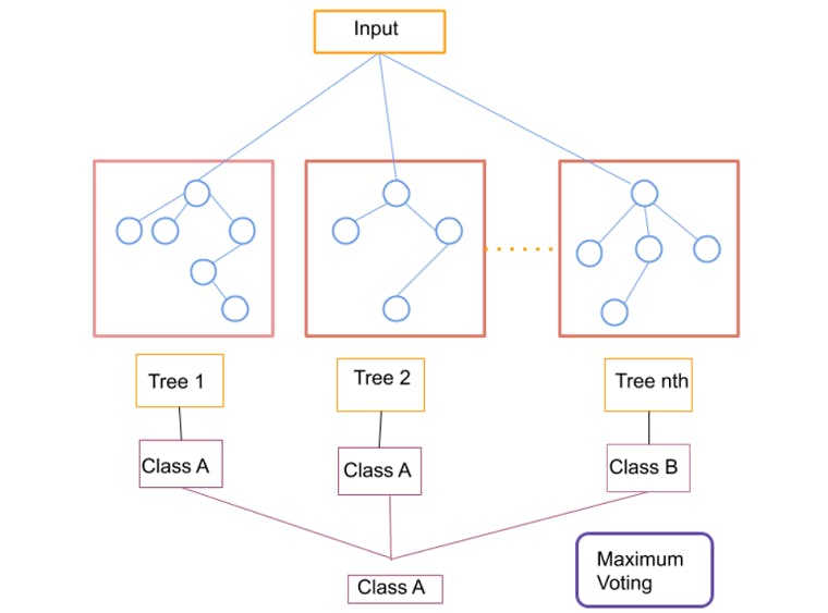
In other words, we can define a random forest as an ensemble ML algorithm. Or an ensemble of decision trees.

Before we head on to learn how to develop random forest ensemble in Python, let’s examine the term “decision trees” which lays the foundation for this model.

Decision trees

To understand this in the simplest way, decision trees are models that are defined by data features. These are built with a set of boolean conditions, which are represented in the form of a binary tree.

Let’s create a sample dataset where every one of 100 samples is defined by two features, say X and Y. Assuming the classes to be green, blue, and red, here’s a make_blobs function that will ease the task.

import matplotlib.pyplot as plt
from sklearn.datasets import make_blobs
%matplotlib inline
RANDOM_STATE = 0  # Ensure repeatability when using randomness
COLORS = ["red", "green", "blue"]
FEATURES_NAMES = ["X", "Y"]
features, labels = make_blobs(
    centers=[(-4, 4), (0, -4), (4, 4)],
    random_state=RANDOM_STATE
)
labels_colors = [COLORS[label] for label in labels]
plt.scatter(features[:, 0], features[:, 1], c=labels_colors)
plt.xlabel(FEATURES_NAMES[0])
plt.ylabel(FEATURES_NAMES[1])
plt.show()

Code source

Next, we have to create our tree classifier. Know that all scikit-learn models have the same API for training: fit (features, labels).

from sklearn.tree import DecisionTreeClassifier
decision_tree = DecisionTreeClassifier()
decision_tree.fit(features, labels)
DecisionTreeClassifier(class_weight=None, criterion='gini', max_depth=None,
            max_features=None, max_leaf_nodes=None,
            min_impurity_decrease=0.0, min_impurity_split=None,
            min_samples_leaf=1, min_samples_split=2,
            min_weight_fraction_leaf=0.0, presort=False, random_state=None,
            splitter='best')

Code source

Lastly, we need to investigate the structure of our tree classifier using the graphviz library.

import graphviz
from sklearn.tree import export_graphviz
tree_data = export_graphviz(
    decision_tree=decision_tree,
    out_file=None,
    feature_names=FEATURES_NAMES,
    class_names=COLORS,
    rounded=True,
    filled=True,
    impurity=False
)
tree_graph = graphviz.Source(tree_data)
tree_graph

Code source

Now, let's dig deep into the ensemble method in the random forest algorithm.

Ensemble methods in random forest algorithm

Ensemble methods are meta-algorithms or machine learning methods that build a set of predictive models and offer a single prediction from them.

How does it work?

Several decision trees are created in it and each forms a tree from a distinct bootstrap sample from the given dataset.

Note: A bootstrap is a sample from the given training dataset where it may appear more than one time. It is also known as sampling without replacement.

So, in the ensemble method of the random forest model, it combines different weaker learning models ‌to provide a better prediction capability. This learning models may run sequentially or parallelly. It can also learn from each other and finally compound learning in certain ensemble techniques.

The accuracy of the results from this method is far better than the results from the individual weaker models that were initially combined to create the ensemble model. This enhances the predictive performance and accuracy as demanded.

To summarize, we can say that the greater the variation in the learning models within the ensemble, more robust results will be generated.

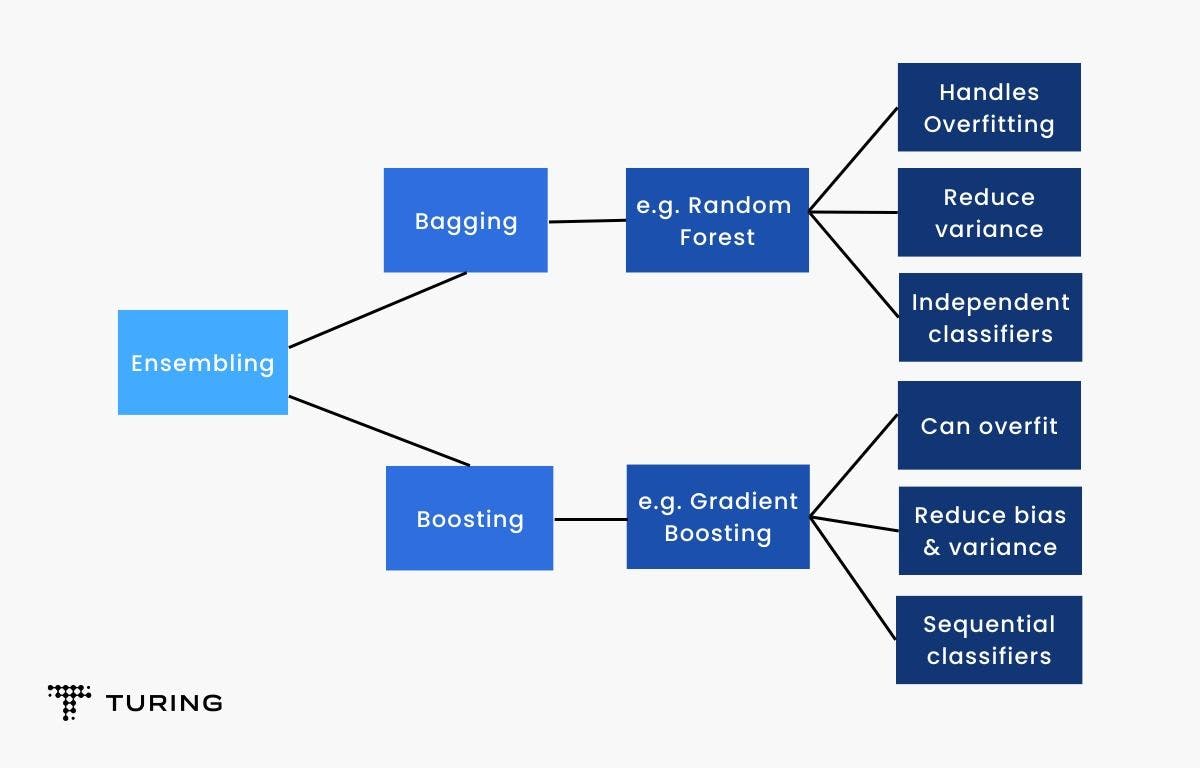
Different types of ensemble models

Bagging and Boosting are some of the renowned ensemble techniques to obtain higher accuracy in results on decision trees. Here’s a pictorial representation to understand the same in detail.

Types of boosting in the ensemble method

1. AdaBoost

Boosting is another type of the ensemble method that deals with the stacking problem of classifiers from the other end. It helps in reducing general bias using several other high-bias models. However, AdaBoost uses multiple weak learners and then cooperatively decides to further empower it.

To sum up, start by building small trees one by one and then focus on any mistakes you have made in the past to ace your procedure under this method.

Fact: AdaBoost uses trees that are shallow, which are often referred to as decision stumps. They only have two leaves and are not used as base learners in the AdaBoost algorithm.

2. Gradient tree boosting

Another member of the boosting family is the gradient tree boosting. This algorithm is laid on the foundation that helps in iteratively finding new trees. It will ultimately lower the loss function (which tells how bad the model is).

It is quite similar to AdaBoost as it is built from a bundle of small trees. However, they are deeper than the decision stumps. The training of individual trees is not identical, but they are trained sequentially. All of them possess similarities to the classification trees, with the only difference being that they are trained to output a real number instead of labeling as an output for a sample.

Fact: Regression trees make up the gradient tree boosting. Each class owns its regression tree and a trained trees offers a result of the probability of which particular sample belongs to the same class. For training, the values used are 1 and 0 only. So, to know if a tree is perfectly trained, ‌you should expect either answer.

Bagging

This ensemble algorithm is known to improve the accuracy of other machine learning algorithms by using a concept called bootstrap.

Since our agenda is to develop a random forest ensemble, let’s dig deep into the bagging technique and decision trees under the ensemble method.

Here’s everything you need to know.

For beginners, bagging can be a daunting task. The scikit-learn Python machine learning library offers the modern version of implementing it in its library. So, before you check it out, confirm if you are using a modern version of the library.

Run the following script to check.

# check scikit-learn version                 
import sklearn                  
print(sklearn.__version__)

Code source

It will provide you with the version of scikit-learn. Your version should be ‌“0.22.1” or higher. If that’s not what you have, ‌upgrade your version.

In the scikit-learn library, there is a module for bagging techniques available for both random forest regression and classification settings.

Let’s understand it with a simple code that is used to apply BaggingRegressor.

from sklearn.ensemble import BaggingClassifier, BaggingRegressor                
regr1 = BaggingRegressor(max_features=13, random_state=1)                
regr1.fit(X_train, y_train)                  
#or           
clf1 = BaggingClassifier(max_features=13, random_state=1)            
clf1.fit(X_train, y_train)

Code source

Note: The syntax does not change with BaggingClassifier and BaggingRegressor and neither does the functioning of the bagging technique. It is only the nature of the target variable in both cases that makes the difference.

Let’s check out the result when we apply the BaggingClassifier to the dataset. Use the following code to see the output.

We will also see what results can be derived by applying the BaggingClassifier to the iris dataset. Run the code given below to see the output.

STEP 1 - Loading the iris data set
from sklearn import datasets

iris = datasets.load_iris()

STEP 2 - Defining the predictors and target variable

X = iris.data               
y = iris.target

STEP 3 - Splitting the data into training and test data
from sklearn.model_selection import train_test_split

X_train, X_test = train_test_split(X, test_size=0.3, random_state=20052017)            
y_train, y_test = train_test_split(y, test_size=0.3, random_state=20052017)

STEP 4 - Importing and fitting the model
from sklearn.ensemble import BaggingClassifier

iris_BC = BaggingClassifier(n_estimators=100, max_features=3, random_state=0)                 
BC = iris_BC.fit(X_train,y_train)

STEP 5 - Calculating the score of the model using the test data
BC.score(X_test,y_test)

Code source

When you run the code, you can find the output to be 0.9555555555555556 that exists in the higher accuracy order.

Random forest ensemble methods are so simple that even a Pigeon can understand them. In this supervised machine learning algorithm, different decision trees yield distinct samples based on which the majority vote for classification and the average for regression are calculated. You just have to get a set of random forest models, aggregate the predictions and there you are with a result fused with accuracy. That’s all!

Here’s a small recap of everything we have learned in this article.

• Decision trees are high variance models that can be rectified by using ensembles.
• With the help of scikit-learn, you can obtain an easy API to train ensemble models and that too, with a standard quality level.
• Ensembling methods are divided into two main groups - Bagging (random forests) and boosting (gradient tree boosting).

We hope this detailed look at the random forest ensemble method development in Python will help you.