A Guide on Word Embeddings in NLP

What is word embedding?

Word embedding or word vector is an approach with which we represent documents and words. It is defined as a numeric vector input that allows words with similar meanings to have the same representation. It can approximate meaning and represent a word in a lower dimensional space. These can be trained much faster than the hand-built models that use graph embeddings like WordNet.

For instance, a word embedding with 50 values holds the capability of representing 50 unique features. Many people choose pre-trained word embedding models like Flair, fastText, SpaCy, and others.

We will discuss it further in the article. Let’s move on to learn it briefly with an example of the same.

The problem

Given a supervised learning task to predict which tweets are about real disasters and which ones are not (classification). Here the independent variable would be the tweets (text) and the target variable would be the binary values (1: Real Disaster, 0: Not real Disaster).

Now, Machine Learning and Deep Learning algorithms only take numeric input. So, how do we convert tweets to their numeric values? We will dive deep into the techniques to solve such problems, but first let’s look at the solution provided by word embedding.

The solution

Word Embeddings in NLP is a technique where individual words are represented as real-valued vectors in a lower-dimensional space and captures inter-word semantics. Each word is represented by a real-valued vector with tens or hundreds of dimensions.

Term frequency-inverse document frequency (TF-IDF)

Term frequency-inverse document frequency is the machine learning algorithm that is used for word embedding for text. It comprises two metrics, namely term frequency (TF) and inverse document frequency (IDF).

This algorithm works on a statistical measure of finding word relevance in the text that can be in the form of a single document or various documents that are referred to as corpus.

The term frequency (TF) score measures the frequency of words in a particular document. In simple words, it means that the occurrence of words is counted in the documents.

The inverse document frequency or the IDF score measures the rarity of the words in the text. It is given more importance over the term frequency score because even though the TF score gives more weightage to frequently occurring words, the IDF score focuses on rarely used words in the corpus that may hold significant information.

TF-IDF algorithm finds application in solving simpler natural language processing and machine learning problems for tasks like information retrieval, stop words removal, keyword extraction, and basic text analysis. However, it does not capture the semantic meaning of words efficiently in a sequence.

Now let’s understand it further with an example. We will see how vectorization is done in TF-IDF.

To create TF-IDF vectors, we use Scikit-learn’s TF-IDF Vectorizer. After applying it to the previous 4 sample tweets, we obtain -

Output of TfidfVectorizer

The rows represent each document, the columns represent the vocabulary, and the values of tf-idf(i,j) are obtained through the above formula. This matrix obtained can be used along with the target variable to train a machine learning/deep learning model.

Let us now discuss two different approaches to word embeddings. We’ll also look at the hands-on part!

Bag of words (BOW)

A bag of words is one of the popular word embedding techniques of text where each value in the vector would represent the count of words in a document/sentence. In other words, it extracts features from the text. We also refer to it as vectorization.

To get you started, here’s how you can proceed to create BOW.

• In the first step, you have to tokenize the text into sentences.
• Next, the sentences tokenized in the first step have further tokenized words.
• Eliminate any stop words or punctuation.
• Then, convert all the words to lowercase.
• Finally, move to create a frequency distribution chart of the words.

We will discuss BOW with proper example in the continuous bag of word selection below.

Word2Vec

Word2Vec method was developed by Google in 2013. Presently, we use this technique for all advanced natural language processing (NLP) problems. It was invented for training word embeddings and is based on a distributional hypothesis.

In this hypothesis, it uses skip-grams or a continuous bag of words (CBOW).

These are basically shallow neural networks that have an input layer, an output layer, and a projection layer. It reconstructs the linguistic context of words by considering both the order of words in history as well as the future.

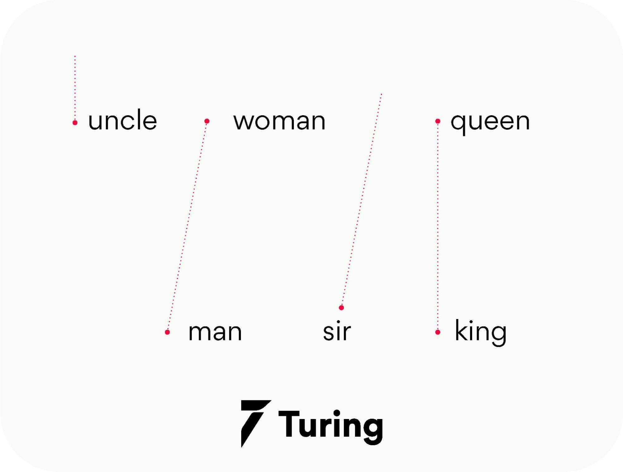
The method involves iteration over a corpus of text to learn the association between the words. It relies on a hypothesis that the neighboring words in a text have semantic similarities with each other. It assists in mapping semantically similar words to geometrically close embedding vectors.

It uses the cosine similarity metric to measure semantic similarity. Cosine similarity is equal to Cos(angle) where the angle is measured between the vector representation of two words/documents.

• So if the cosine angle is one, it means that the words are overlapping.
• And if the cosine angle is a right angle or 90°, It means words hold no contextual similarity and are independent of each other.

To summarize, we can say that this metric assigns similar vector representations to the same boards.

Two variants of Word2Vec

Word2Vec has two neural network-based variants: Continuous Bag of Words (CBOW) and Skip-gram.

1. CBOW - The continuous bag of words variant includes various inputs that are taken by the neural network model. Out of this, it predicts the targeted word that closely relates to the context of different words fed as input. It is fast and a great way to find better numerical representation for frequently occurring words. Let us understand the concept of context and the current word for CBOW.

In CBOW, we define a window size. The middle word is the current word and the surrounding words (past and future words) are the context. CBOW utilizes the context to predict the current words. Each word is encoded using One Hot Encoding in the defined vocabulary and sent to the CBOW neural network.

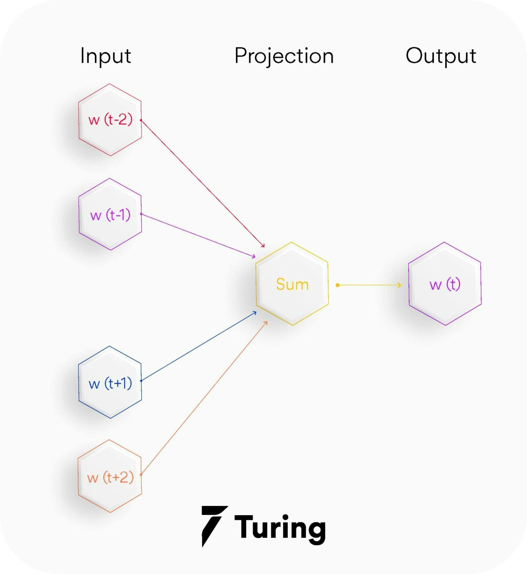
The hidden layer is a standard fully-connected dense layer. The output layer generates probabilities for the target word from the vocabulary.

As we have discussed earlier about the bag of words (BOW) and it being also termed as vectorizer, we will take an example here to clarify it further.

Let's take a small part of disaster tweets, 4 tweets, to understand how BOW works:-

‘kind true sadly’,

‘swear jam set world ablaze’,

‘swear true car accident’,

‘car sadly car caught up fire’

To create BOW, we use Scikit-learn’s CountVectorizer, which tokenizes a collection of text documents, builds a vocabulary of known words, and encodes new documents using that vocabulary.

Output of CountVectorizer

Here the rows represent each document (4 in our case), the columns represent the vocabulary (unique words in all the documents) and the values represent the count of the words of the respective rows.

In the same way, we can apply CountVectorizer to the complete training data tweets (11,370 documents) and obtain a matrix that can be used along with the target variable to train a machine learning/deep learning model.

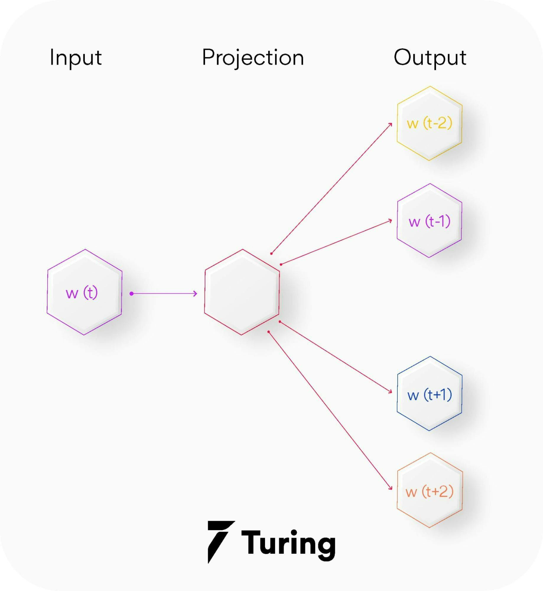
2. Skip-gram — Skip-gram is a slightly different word embedding technique in comparison to CBOW as it does not predict the current word based on the context. Instead, each current word is used as an input to a log-linear classifier along with a continuous projection layer. This way, it predicts words in a certain range before and after the current word.

This variant takes only one word as an input and then predicts the closely related context words. That is the reason it can efficiently represent rare words.

The end goal of Word2Vec (both variants) is to learn the weights of the hidden layer. The hidden consequences will be used as our word embeddings!! Let's now see the code for creating custom word embeddings using Word2Vec-

Import Libraries
from gensim.models import Word2Vec
import nltk
import re
from nltk.corpus import stopwords

Preprocess the Text

#Word2Vec inputs a corpus of documents split into constituent words.
corpus = []
for i in range(0,len(X)):
 tweet = re.sub(“[^a-zA-Z]”,” “,X[i])
 tweet = tweet.lower()
 tweet = tweet.split()
 corpus.append(tweet)

Here is the exciting part! Let's try to see the most similar words (vector representations) of some random words from the tweets -
model.wv.most_similar(‘disaster’)

Output -

List of tuples of words and their predicted probability
The embedding vector of ‘disaster’ -

List of tuples of words and their predicted probability
The embedding vector of ‘disaster’ -

dimensionality = 100

Challenges with the bag of words and TF-IDF

Now let’s discuss the challenges with the two text vectorization techniques we have discussed till now.

In BOW, the size of the vector is equal to the number of elements in the vocabulary. If most of the values in the vector are zero then the bag of words will be a sparse matrix. Sparse representations are harder to model both for computational reasons and also for informational reasons.

Also, in BOW there is a lack of meaningful relations and no consideration for the order of words. Here’s more that adds to the challenge with this word embedding technique.

• Massive amount of weights: Large amounts of input vectors invite massive amounts of weight for a neural network.
• No meaningful relations or consideration for word order: The bag of words does not consider the order in which the words appear in the sentences or a text.
• Computationally intensive: With more weight comes the need for more computation to train and predict.

While the TF-IDF model contains the information on the more important words and the less important ones, it does not solve the challenge of high dimensionality and sparsity, and unlike BOW it also makes no use of semantic similarities between words.

GloVe: Global Vector for word representation

GloVe method of word embedding in NLP was developed at Stanford by Pennington, et al. It is referred to as global vectors because the global corpus statistics were captured directly by the model. It finds great performance in world analogy and named entity recognition problems.

This technique reduces the computational cost of training the model because of a simpler least square cost or error function that further results in different and improved word embeddings. It leverages local context window methods like the skip-gram model of Mikolov and Global Matrix factorization methods for generating low dimensional word representations.

Latent semantic analysis (LSA) is a Global Matrix factorization method that does not do well on world analogy but leverages statistical information indicating a sub-optimal vector space structure.

On the contrary, the skip-gram method performs better on the analogy task. However, it does not utilize the statistics of the corpus properly because of no training on global co-occurrence counts.

So, unlike Word2Vec, which creates word embeddings using local context, GloVe focuses on global context to create word embeddings which gives it an edge over Word2Vec. In GloVe, the semantic relationship between the words is obtained using a co-occurrence matrix.

Consider two sentences -

I am a data science enthusiast

I am looking for a data science job

The co-occurrence matrix involved in GloVe would look like this for the above sentences -

Window Size = 1

Each value in this matrix represents the count of co-occurrence with the corresponding word in row/column. Observe here - this co-occurrence matrix is created using global word co-occurrence count (no. of times the words appeared consecutively; for window size=1). If a text corpus has 1m unique words, the co-occurrence matrix would be 1m x 1m in shape. The core idea behind GloVe is that the word co-occurrence is the most important statistical information available for the model to ‘learn’ the word representation.

Let's now see an example from Stanford’s GloVe paper of how the co-occurrence probability rations work in GloVe. “For example, consider the co-occurrence probabilities for target words ice and steam with various probe words from the vocabulary. Here are some actual probabilities from a corpus of 6 billion words:”

Here,

Let's take k = solid i.e, words related to ice but unrelated to steam. The expected Pik /Pjk ratio will be large. Similarly, for words k which are related to steam but not to ice, say k = gas, the ratio will be small. For words like water or fashion, which are either related to both ice and steam or neither to both respectively, the ratio should be approximately one.

The probability ratio is able to better distinguish relevant words (solid and gas) from irrelevant words (fashion and water) than the raw probability. It is also able to better discriminate between two relevant words. Hence in GloVe, the starting point for word vector learning is ratios of co-occurrence probabilities rather than the probabilities themselves.

Enough of the theory. Time for the code!

Import Libraries
import nltk
import re
from nltk.corpus import stopwords
from glove import Corpus, Glove
Text Preprocessing
#GloVe inputs a corpus of documents splitted into constituent words
corpus = []
for i in range(0,len(X)):
 tweet = re.sub(“[^a-zA-Z]”,” “,X[i])
 tweet = tweet.lower()
 tweet = tweet.split()
 corpus.append(tweet)
Train the word Embeddings
corpus = Corpus()
corpus.fit(text_corpus,window = 5)
glove = Glove(no_components=100, learning_rate=0.05)
#no_components = dimensionality of word embeddings = 100
glove.fit(corpus.matrix, epochs=100, no_threads=4, verbose=True)
glove.add_dictionary(corpus.dictionary)
Find most similar -
glove.most_similar(“storm”,number=10)

Output -

List of tuples of words and their predicted probability

BERT (Bidirectional encoder representations from transformers)

This natural language processing (NLP) based language algorithm belongs to a class known as transformers. It comes in two variants namely BERT-Base, which includes 110 million parameters, and BERT-Large, which has 340 million parameters.

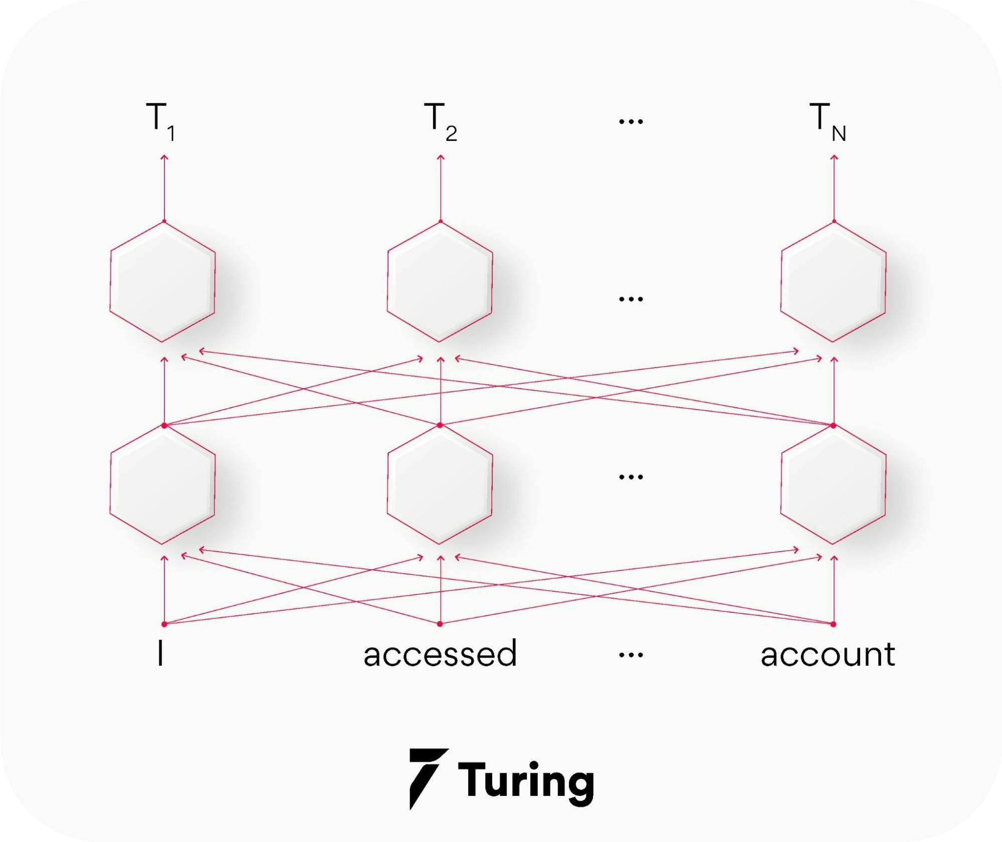
It relies on an attention mechanism for generating high-quality world embeddings that are contextualized. So when the embedding goes through the training process, they are passed through each BERT layer so that its attention mechanism can capture the word associations based on the words on the left and those on the right.

It is an advanced technique in comparison to the discussed above as it creates better word embedding. The credit goes to the pre-trend model on Wikipedia data sets and massive word corpus. This technique can be further improved for task-specific data sets by fine-tuning the embeddings.

It finds great application in language translation tasks.

Conclusion

Word embeddings can ‌train deep learning models like GRU, LSTM, and Transformers, which have been successful in NLP tasks such as sentiment classification, name entity recognition, speech recognition, etc.

Here’s a final checklist for a recap.

• Bag of words: Extracts features from the text
• TF-IDF: Information retrieval, keyword extraction
• Word2Vec: Semantic analysis task
• GloVe: Word analogy, named entity recognition tasks
• BERT: language translation, question answering system

In this blog, we discussed the two techniques for vectorizations in NLP: the Bag of Words and TF-IDF, their drawbacks, and how word-embedding techniques like GloVe and Word2Vec overcome their drawbacks by dimensionality reduction and context similarity. With all said above, you would have a better understanding of how word embeddings benefits your day-to-day life as well.