How and Where to Apply Feature Scaling in Python?

Transforming your data to make it fit with a specific scale will improve the performance of your machine learning (ML) model. Since ML is a combination of different elements, it’s important to choose the right proportion of each to arrive at the best combination. Similarly, with machine learning algorithms, you can bring all the features together and scale them so that they become a significant item that doesn’t impact the model just because it has a higher magnitude.

Feature scaling and its common processes

Feature scaling is one of the most crucial steps that you must follow when preprocessing data before creating a machine learning model. With feature scaling, you can make a stronger difference between a robust and weaker ML model. It has two common techniques that help it to work, standardization and normalization.

1. Standardization

Standardization is a technique where the values are positioned around the mathematical average with a unit standard deviation. It means that the mathematical average of the attribute will become zero and the result of the distribution will have a unit standard deviation.

The formula for standardization is:

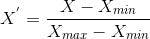
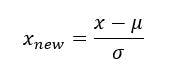
The formula for standardization is:

Here,

is the mathematical average and

is the standard deviation of the feature values. With standardization, the values are not restricted to a specific range.

2. Normalization

Normalization is a scaling technique where you shift the values and rescale them so they end up between 0 and 1. Normalization is also known as rescaling or min-max scaling.

The formula for normalization is:

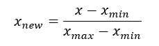
The formula for normalization is:

Here, Xmin and Xmax are the minimum and maximum values of the feature, respectively. So,

• When the value of X is the minimum value, the numerator will be 0, and X’ will be 0.
• When the value of X is the maximum value, the numerator will be equal to the denominator and the value of X’ will be 1.
• When the value of X is between the minimum and maximum values, the value of X’ will be between 0 and 1.

Choosing between standardization and normalization

Normalization is mainly used when you want to keep values between 0 and 1, or -1 and 1. Standardization transforms data to get a zero mean and a variance of 1. It makes data unitless.
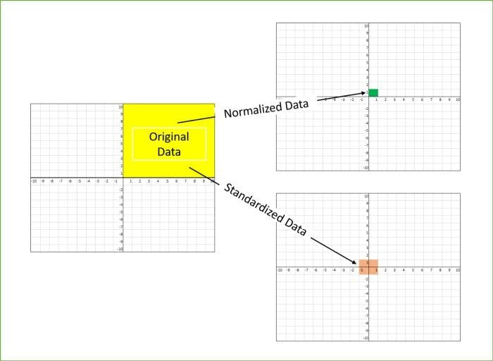
The diagram below shows how data looks when scaled with the X-Y plane:

Image source

Why is scaling needed?

Feature scaling assists with the calculation of various attributes between data. ML algorithms are sensitive to the ‘relative scales of features’, which occur when using the numeric values of features rather than their rank.

As in neural networks and other algorithms, scaling is a vital step when seeking faster convergence. Since the range of raw data values differs widely, objective functions will not work well without normalization. For instance, most classifiers will calculate the distance between two points by the distance. When one of the features has a broader range of values, the distance rules this feature. Hence, the range of all features should be normalized so that each can contribute to the final distance.

When the above instances are not satisfied, you will still need to rescale your features when the algorithm expects a certain scale or saturation. A neural network with saturation activity is a good example to explain this. The rule of thumb for such cases is computing the distance or assuming normality by scaling features.

Machine learning algorithms work only on numbers and not the variables that the numbers represent. For example, 10 is a number that can represent anything from weight to time, which is easier for humans to understand. However, the machine treats both variables as 10, so training it to understand the significance/meaning of numbers is important. This is where feature scaling comes into play.

Feature scaling brings each feature on the same criteria without any honest standing. Meanwhile, algorithms like neural networks have a gradient descent that converges rapidly with feature scaling. In the case of sigmoid activation in a neural network, scaling helps lower the rate of saturation.

When is scaling needed?

Here are some sample algorithms where feature scaling is required:

• K-nearest neighbors (KNN) with a Euclidean distance will help measure data of sensitive magnitude so that all the features will weigh equally.
• K-means with a Euclidean distance is required to measure feature scaling.
• Principal component analysis (PCA) is another area where feature scaling is vital. With PCA, you can get the features with maximum variance. The variance is high for higher magnitude and skews the PCA towards the higher magnitude features.
• Gradient descent can be hastened with scaling as theta descends quickly on smaller ranges, slowly on larger ranges, and oscillates inefficiently down to the optimum when the variables are uneven.

Algorithms that rely entirely on rules do not require scaling. This is because they will not be affected by any transformations in the variables. Scaling is a monotonic transformation. For instance, CART, gradient boosted decision trees, and other related tree-based algorithms utilize rules and do not require normalization.

There is no point in activating feature scaling in linear discriminant analysis (LDA ) and Naïve Bayes as they are designed to handle this and give weights to features accordingly. There are also certain key factors to note: variable scaling and mean centering will not affect the covariance matrix while standardizing will affect the covariance.

How to apply feature scaling

There are several ways to apply feature scaling:

1. Min-max
2. MaxAbs
3. Quantile transformer
4. Standard
5. Robust
6. Unit vector
7. Power transformer

1. Min-max scaling

The min-max scaler formula is:

The min-max scaler formula is:

With this estimation scale, each feature can be translated separately within the range provided on the training set. The min-max scaler allows you to shrink the data within the range of -1 to 1 when there can be negative values.

The range for training the set can be (0,1), (0,5), or (-1,1). The scaling responds at its best when the standard deviation is small and when a distribution is not Gaussian. These scalers are also sensitive to outliers.

2. MaxAbs scaling

MaxAbs scaling lets you scale each feature with its maximum absolute value. This will estimate the scales and translate the feature uniquely so that the maximum value of each feature is set to 1. It doesn’t move the data and will not destroy any sparsity. When the data is solely positive, the scaler acts like that of a min-max scaler, so it is affected by the presence of significant outliers.

3. Quantile transformer scaling

Also known as a rank scaler, quantile transformer scaling involves transforming features with the help of quantiles information. It transforms features by following a structured distribution. Thus, for a said feature, this transformation spreads throughout the most frequent values.

This scaling technique lets you reduce the impact of marginal outliers, which makes it a robust scheme. The combined distribution function of a feature is used for projecting the original values. This transformation is non-linear and may distort linear correlations between variables measured at the same scale. However, those that render variables measured at different scales are more directly comparable.

4. Standard scaling

The standard scaler formula is:

The standard scaler formula is:

Standard scaler will assume data that is normally distributed within each feature and will scale them so that the distribution will be around 0, with a standard deviation of 1. Computing the relevant details on the samples in the training set is crucial when centering and scaling features independently on each feature. This scaler is not suitable when data is not distributed.

5. Robust scaling

As the name suggests, this scaler is robust to outliers. When data contains many outliers, scaling using the standard and mean deviation of data will not work well. This scaler removes the median while scaling the data according to the quantile range.

The interquartile range is the range between the first and third quartiles. The centering and scaling figures of this scaler are based on the percent and will not be influenced by a few huge marginal outliers. Note that the outliers are still present in the transformed data. A non-linear transformation is required when a separate outlier clipping is necessary.

6. Unit vector scaling

The unit vector scaler formula is:

The unit vector scaler formula is:

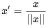
Unit vector scaling is done keeping in mind the whole feature vector in a unit length. This normally requires dividing each component by the Euclidean length of the vector. In certain applications, it can be practical to use the L1 norm of the feature vector.

Like min-max scaling, the unit vector technique will produce values that range between 0 and 1. It is useful when dealing with features with hard boundaries.

7. Power transformer scaling

Power transformer scaling is a family of monotonic, parametric transformations that apply to making data more Gaussian-like. It is useful for modeling issues related to the unpredictability of a variable that is incapable across the range of situations where it is usually anticipated. The power transformer will find the optimal scaling factor for stabilizing variance and minimizing skewness over maximum estimation.

Currently, Sklearn’s implementation of power transformer scaling supports Box-Cox and Yeo-Johnson transformations. The optimal parameter for stabilizing variance and minimizing skewness is by estimating over maximum estimation. Box-Cox transformation requires its input data to be strictly positive, whereas you can have both positive and negative data with Yeo-Johnson.

As is now clear, feature scaling is a vital step in machine learning preprocessing. Since deep learning needs feature scaling for quicker convergence, it is important to choose the right type. Keep in mind, however, that like other ML steps, feature scaling is a trial process and a final solution.