Understanding the Complete Life Cycle of a Data Science Project

The modern lifestyle is generating data at unparalleled speed. Apps, websites, smartphones, etc. create data at an individual level. This is then gathered and stored in giant servers and datastores that cost these companies thousands, if not millions of dollars, in maintenance and upkeep.

But why go to such lengths?

Because this vast storage of data is nothing less than a gold mine - if you can get a hold of someone who’s learned the art of extracting stories and patterns from the gigantic pile of unstructured words and numbers.

Enter the data scientist. Professionals who can make a world of difference with this data. They sort through the information, analyze it, create bars and graphs, draw inferences, and then relay their findings to decision-makers.

A business grows by taking calculated risks, and data scientists are the ones who calculate that risk.

In this article, we shall learn about the complete life cycle of a data science project.

Let’s get started.

The Data Science team

As organizations expand, the data generated increases, leading to a more sophisticated approach to the data science process. To now achieve their goals, companies have to hire more individuals with a specific skill set. This leads to the creation of a data science team that might consist of:

• Data scientist
• Data analyst
• Data engineer
• Data architect
• Machine learning engineer
• Business analyst
• Data translator
• Data visualization developer

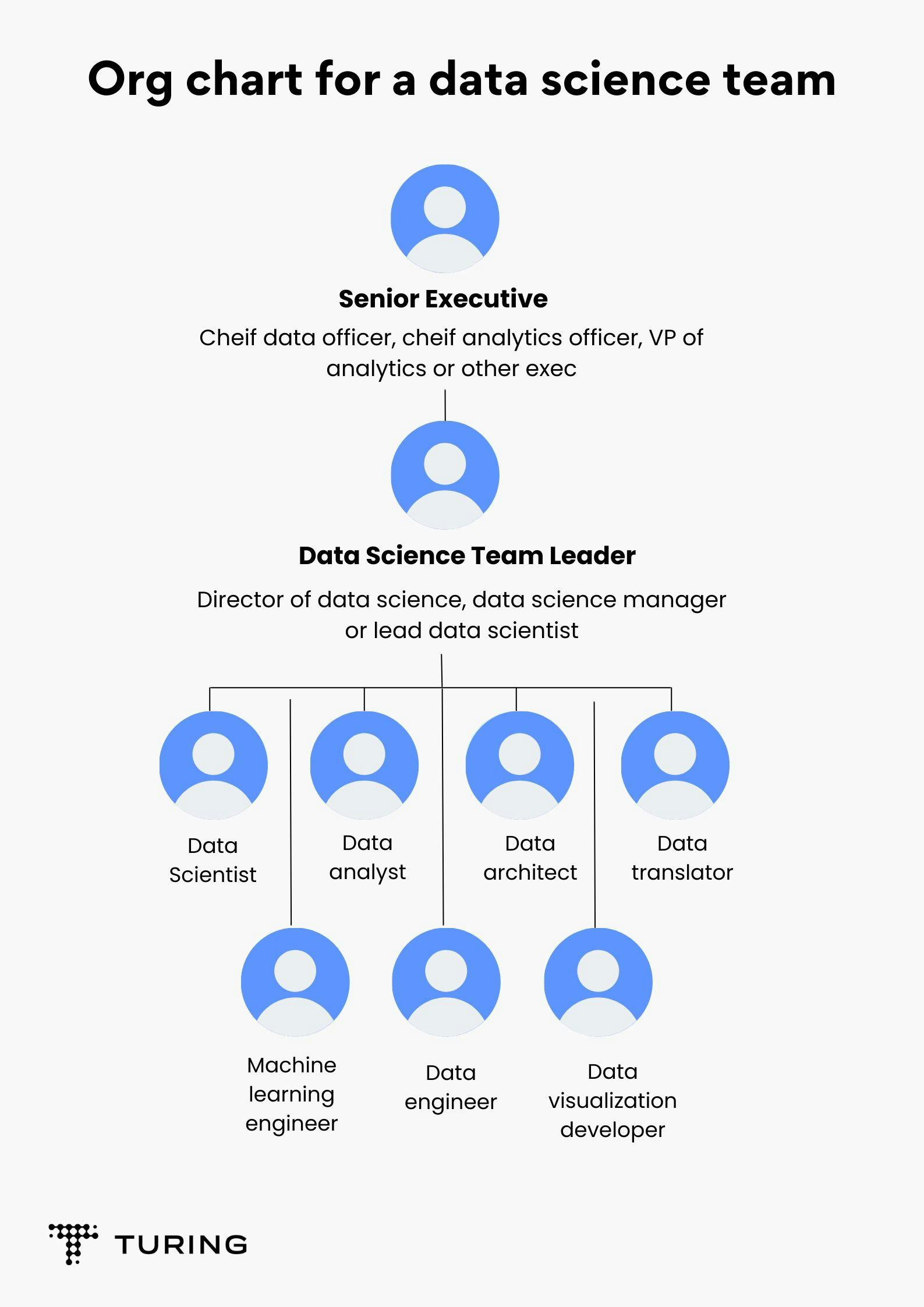
All the members of this team have to work together. And each has something to offer at every stage of the data science project.

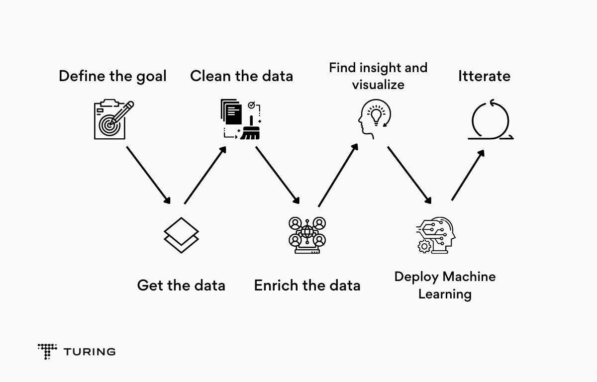
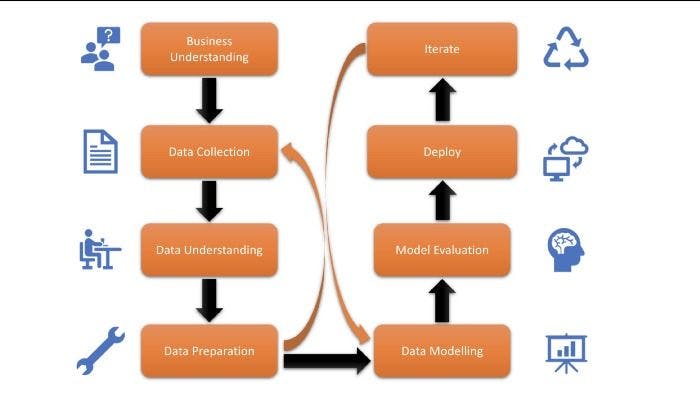
The Data Science project life cycle

A data science project is a very long and exhausting process. In a real-life business scenario, it takes months, even years, to get to the endpoint where the developed model starts to show results.

To help readers understand the process more clearly, we will use a sample project to gain a working understanding of what goes on under the hood.

Step 1: Business understanding - asking the right questions

This step is necessary for finding a clear objective around which all the other steps will be structured. Why? Because a data science project revolves around the needs of the client or the firm.

Let’s suppose our client is a famous Indian company, Reliance Industries Limited. It has approached us to find the future projections of its stock price.

A business analyst is usually the one responsible for gathering all the necessary details from the client. The questions have to be precise, and sometimes help can be outsourced from domain experts to further our understanding of the client’s business.

Once we have all the relevant information and a game plan, it’s time to mine the gold, i.e., the data.

Step 2: Data collection - finding the right data

Step 2 starts with us finding all the right sources for relevant data. The client may be storing data themselves and want us to analyze it. In the absence of that, however, several other sources are used like server logs, digital libraries, web scraping, social media, etc.

For our project, we shall use Yahoo Finance to get the historical data of Reliance stock (RELIANCE.NS). The data can be downloaded easily.

Image source

Image source

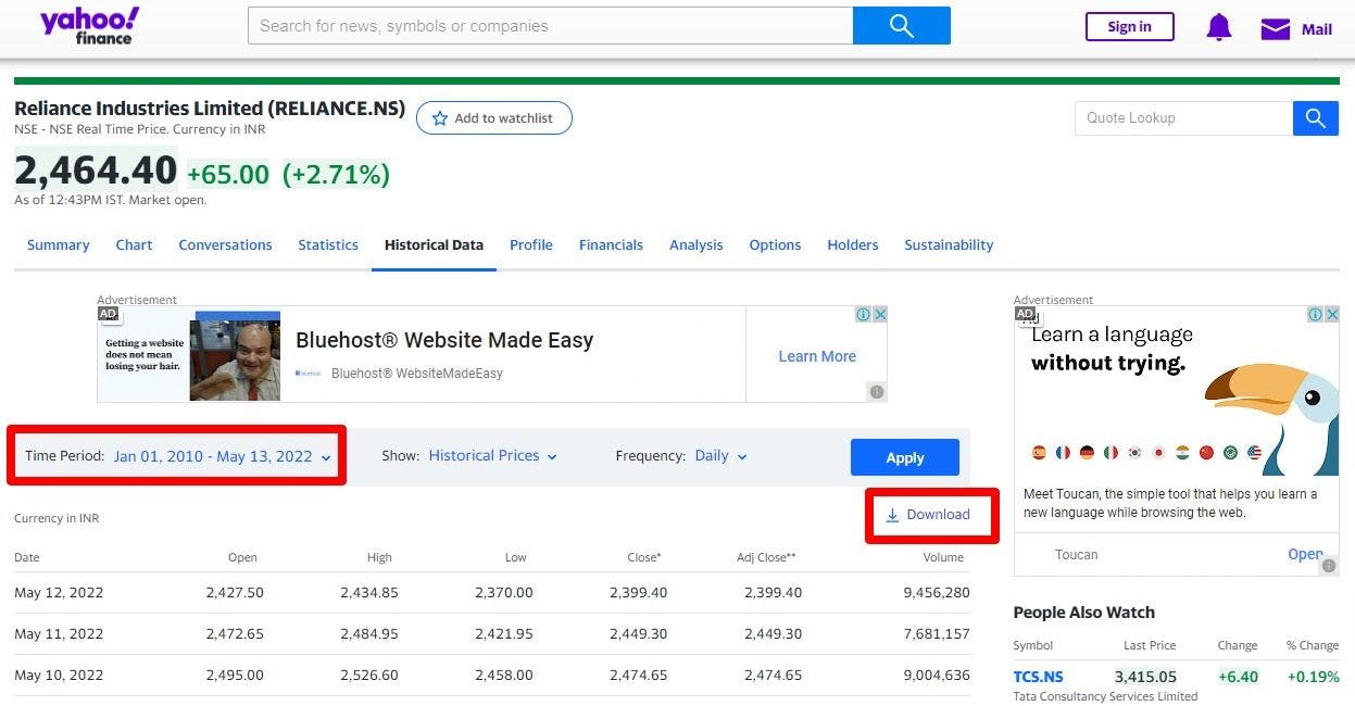
We get a CSV file.

Note: Since the scope of this article is limited, we’ve taken data from just one source. In a real-life project, multiple data sources are considered and the analysis is done using all sorts of structured and unstructured data.

Step 3: Data preparation - order from chaos

This step is arguably the most important because this is where the magic happens. After gathering the necessary data, we move on to the grunt work.

All the different datasets are merged accordingly, the datasets are cleaned, unnecessary features removed and made more structured, missing values are dealt with, redundancy is eliminated, and preliminary tests are done with the data in order to evaluate the direction of the project.

Exploratory data analysis (EDA) is also performed in this step. Using visual aids such as bar plots, graphs, pie charts, etc., helps the team to visualize trends, patterns, and anomalies.

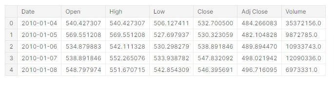
In this step, we load the data in our preferred environment. For this article, we shall use Jupyter Notebook with Python.

Importing libraries

import numpy as np
import pandas as pd
from datetime import datetime
from sklearn.linear_model import LinearRegression
import matplotlib.pyplot as plt

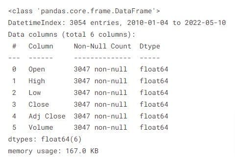
Loading data

df = pd.read_csv('../input/relianceanalysis/RELIANCE.csv')
df.head()

out:

#changing the 'Date' column to datetime objects
df['Date'] = pd.to_datetime(df['Date'])

df.info()

out:

Counting null values:

variables = df.columns
code block

out:

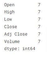
Since there are only 7 null values for each column, out of 3000+ entries, we can safely remove these rows since they don't hold much weightage.

df.dropna(axis = 0, inplace = True)

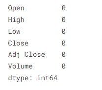
Let’s check again:

variables = df.columns
df.isnull().sum().loc[variables]

out:

Exploratory data analysis

Let’s find the correlation between different features using a custom function:

def correlation(df,Var, n_row, n_col):
fig = plt.figure(figsize=(8,6))
fig = plt.figure(figsize=(8,6))
#fig = plt.figure(figsize=(14,9))
for i, var in enumerate(Var):
ax = fig.add_subplot(n_row,n_col,i+1)
at = df.loc[:,var]
ax.scatter(df["Adj Close"], at, c = next(colors))
ax.set_xlabel("Adj Close")
ax.set_ylabel("{}".format(var))
ax.set_title(var +" vs price")
fig.tight_layout()
plt.show()

And here are our correlation plots:

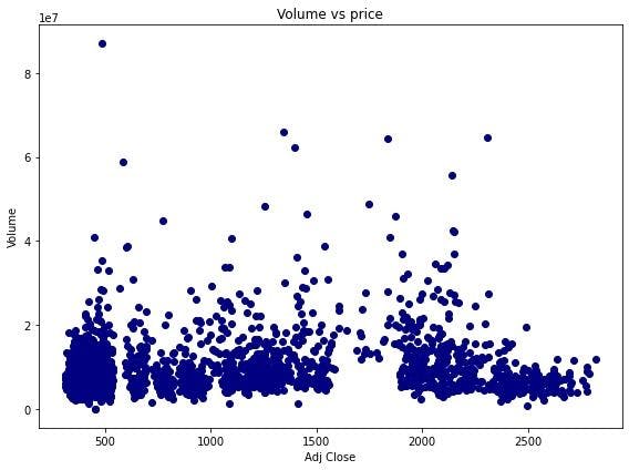
Volume vs Close Price

variables = df.columns[-1:]
correlation(df,variables,1,1)

Open, High, Low, Close vs Adj Close:

variables =df.columns
correlation(df,variables,3,3)

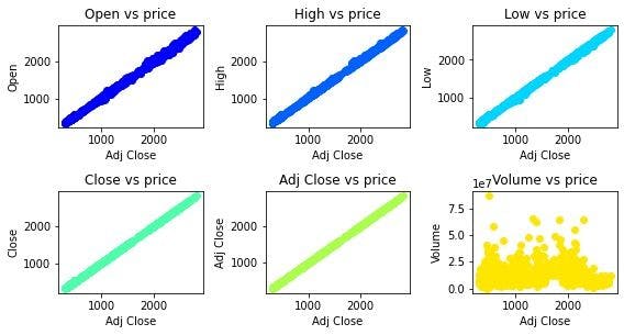
Adj Close is the target feature that we shall predict using a simple linear regression model. From the above scatter plots, we can see that there’s a clear linear relationship between ‘Adj Price’ and all the other features, except ‘Volume’.

Here are the correlation values of Adj Close with the rest of the features:

df.corr()['Adj Close'].loc[variables]

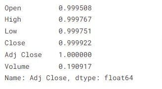
We now know which features to focus on and which to ignore while building our model.
This right here is the main goal of Step 3: to find the right features to help determine the end goal more precisely.

Step 4: Data modeling - organizing the data

Data modeling is at the core of a data science project. The data we have is now organized into the proper format that will be fed into the model. The model follows its algorithm and gives the desired output.

Most ML problems can be divided into three categories: regression problems, classification problems, and clustering problems.

After selecting the type, we choose the particular algorithm that we see fit to use. If the results are not as good as expected, we finetune these models and start the training all over again. It’s an iterative process, one that we repeat until we find our optimal model.

For our project, we’ve selected simple linear regression:

Feature engineering

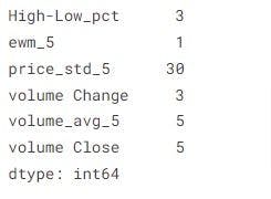
Adding new features:

df['High-Low_pct'] = (df['High'] - df['Low']).pct_change()
df['ewm_5'] = df["Close"].ewm(span=5).mean().shift(periods=1)
df['price_std_5'] = df["Close"].rolling(center=False,window= 30).std().shift(periods=1)

df['volume Change'] = df['Volume'].pct_change()
df['volume_avg_5'] = df["Volume"].rolling(center=False,window=5).mean().shift(periods=1)
df['volume Close'] = df["Volume"].rolling(center=False,window=5).std().shift(periods=1)

Some of the entries have NaN and inf values since there are a lot of calculations in the previous step. We get rid of them by:

# Replacing infinite with nan
df.replace([np.inf, -np.inf], np.nan, inplace=True)
df.isnull().sum().loc[variables]

Dropping all the NULL values:

df.dropna(axis=0,inplace = True)
df.isnull().sum().loc[variables]

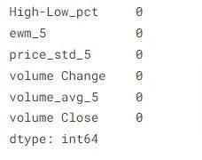
Our dataset is now ready. But first, we split it into train and test data to evaluate our model later:

from sklearn.model_selection import train_test_split
X_train, X_test, Y_train, Y_test = train_test_split(X, Y)

Linear Regression

lr = LinearRegression()
lr.fit(X_train,Y_train)
close_predictions = lr.predict(X_test)

Now, let’s compare 'Y-test' and ‘close-predictions’ to see the accuracy of our model:

lr.score(X_test,Y_test)
0.9980827892628463

Even without tuning any metrics, we can achieve almost 99.9% accuracy!

Here are the first 10 values compared:

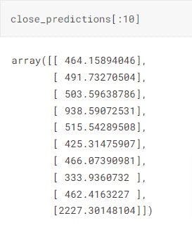
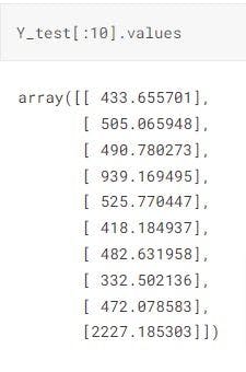
As we can see, our simple linear regression model performs quite well. Though there is a slight chance of overfitting, we can ignore that for the sake of not overcomplicating our example.

We are now ready for the next and final step.

Step 5: Model deployment - not the end

If the model is a success following rigorous testing, it is deployed into the real world. It will work with real data and real clients where anything could go wrong at any minute. Hence, the need to evaluate and further finetune it.

Image source

Image source

As mentioned, a professional data science project is an iterative process. Obtaining feedback from clients and making the model more robust will help it make better and more precise decisions in the future - helping both organizations and clients to remain in business.